Parametrized Surfaces: Dynamic Exploration and Geometric Construction

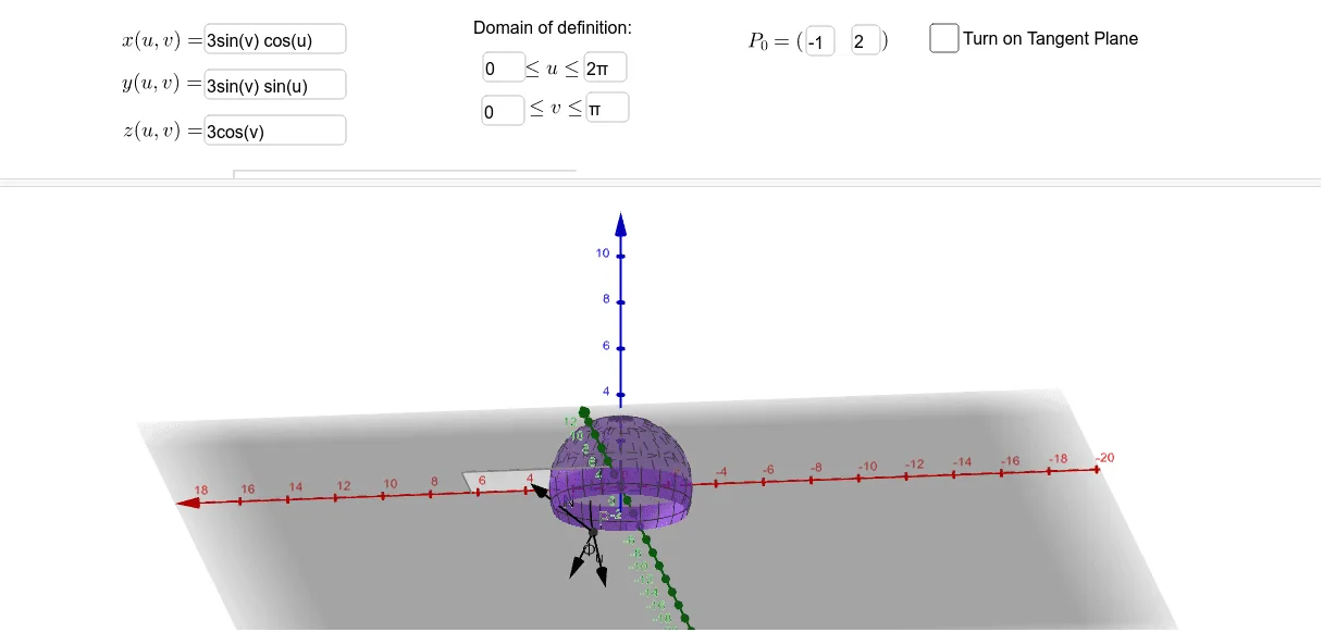
This GeoGebra example demonstrates how to construct and explore parametrized surfaces interactively, visualizing points on the surface, tangent vectors, normal vectors, and partial derivatives. Core mathematical concepts include parametric equations, vector calculus (partial derivatives), tangent planes and normals, and the interaction between the surface and its parameter grid. Construction highlights: the Surface command defines the parametric surface, CurveCartesian draws parameter curves, Derivative computes partial derivatives, Vector and OrthogonalPlane build tangent vectors and tangent planes, while multiple InputBoxes and sliders allow dynamic adjustment of parameters u0, v0 and surface coefficients for real-time exploration. Suitable for university-level calculus, multivariable functions, or differential geometry courses, as well as advanced high school mathematics for intuitive understanding.