
Parametric Equations on a Basketball
Loading the math board and drawing, please wait…
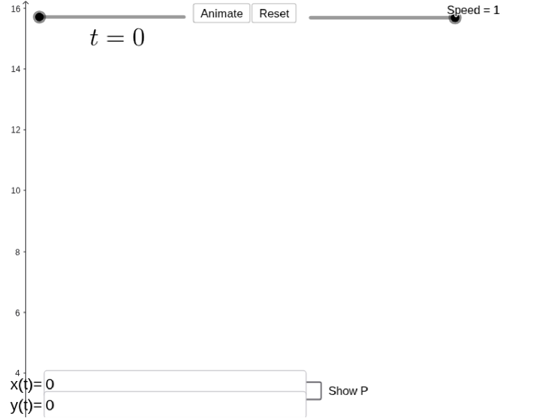
This example demonstrates the parametric equations of a point on a basketball. It involves parametric equations and 3D geometry. Using commands like CurveCartesian, Rotate, and Textfield, the point on the basketball surface can be constructed. Suitable for high school mathematics education, particularly for learning coordinate geometry and parametric equations.
GeoGebra Commands & Parameters
CurveCartesian(((24 * t) * cos(π / 4)), (-16 * t^(2)) + ((24 * t) * sin(π / 4)) + 8, t, 0, p) → aRotate(O + (0, 0.4), (Spin * p), O) → PCurveCartesian(((24 * t) * cos(π / 4)) - (0.4 * sin((Spin * t))), (-16 * t^(2)) + ((24 * t) * sin(π / 4)) + 8 + (0.4 * cos((Spin * t))), t, 0, p) → bCurveCartesian(f(t), g(t), t, 0, p) → cTextfield(f) → inputBox1Textfield(g) → inputBox2Rotate(Dilate[O + (-1, -1), k, O], (Spin * p), O) → ARotate(Dilate[O + (1, -1), k, O], (Spin * p), O) → B
AI Drawing Prompt Reference
Draw a 3D basketball with a moving point on its surface. The basketball is centered at the origin, and its surface is defined by parametric equations. A parabolic trajectory starts from the bottom and curves upward while rotating around the ball. A small sphere moves along this path, and a rotating rectangular frame (representing texture or reference lines) spins around the ball. Two input boxes are shown to adjust the parametric equations. The scene illustrates how parametric equations describe 3D curve motion.
The prompt above was compiled from the original drawing commands and is for reference only.