
Optical Inequality
Loading the math board and drawing, please wait…
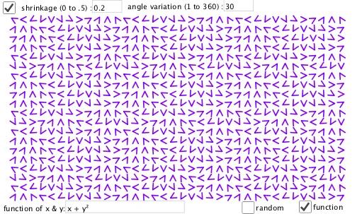
This example demonstrates an optical inequality, involving geometric transformations and function graphs. Users can dynamically adjust parameters to observe the geometric meaning of the inequality using commands like PolyLine, Textfield, and Sequence. Suitable for high school mathematics education and research.
GeoGebra Commands & Parameters
PolyLine(A + spc, A + (1 - spc, 0.5), A + (spc, 1 - spc)) → fTextfield(spc) → InputBox1Sequence(Sequence[Random[0, 360 / ang], i, 1, rx], j, 1, ry) → M_1Sequence(Sequence[Translate[Rotate[f, ((ang * Element[M_a, j, i]))°, A + 0.5], (i - 1, j - 1)], i, 1, rx], j, 1, ry) → L_1Textfield(ang) → InputBox2Sequence(Sequence[g(i, j), i, 1, rx], j, 1, ry) → M_2Textfield(g) → InputBox3Sequence(Sequence[Translate[Rotate[f, ((ang * Element[M_2, j, i]))°, A + 0.5], (i - 1, j - 1)], i, 1, rx], j, 1, ry) → L_2
AI Drawing Prompt Reference
Draw a geometric illustration of an optical inequality, featuring a polygon formed by three points and two grids generated by rotating and translating this polygon. Adjust parameters dynamically to observe the effect of geometric transformations, with one parameter controlling the rotation angle and another affecting the grid density. The image should display the original polygon and its two transformed versions, distinguished by color or style, and include labels for key parameter values.
The prompt above was compiled from the original drawing commands and is for reference only.