
One-Dimensional Elastic Collisions
Loading the math board and drawing, please wait…
In collections
Physics Lab
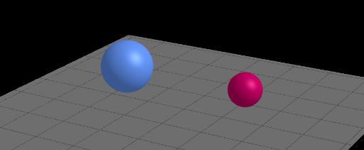
This example demonstrates one-dimensional elastic collisions. Key mathematical concepts include conservation of momentum and kinetic energy. Using GeoGebra commands such as Point, Intersect, Vector, etc., it dynamically shows the velocity changes before and after the collision. Suitable for high school physics and mathematics education.
GeoGebra Commands & Parameters
Point(xAxis) → centermassBPoint(xAxis) → centermassAIntersect(func1i, func2i, 1) → EOrthogonalLine(E, xAxis) → fIntersect(f, xAxis) → FIf(condition01 ≤ 0, func2i, If[0 ≤ x ≤ x(F), func2i(x), func2f(x)]) → qDerivative(q) → q'If(condition01 ≤ 0, func1i, If[0 ≤ x ≤ x(F), func1i, func1f]) → pDerivative(p) → p'LaTeX(condition01, true, true) → text1LaTeX(e, true, true) → text2Circle(centermassA, m1 / 2) → cCircle(centermassB, m2 / 2) → dIf((m1 > 6) ∨ (m2 > 6), -5.5, -3) → groundSurface((((abs(x(A) - x(A')) + bfactor) * cos(u)) * sin(v)) + x(A'), (((abs(x(A) - x(A')) + bfactor) * sin(u)) * sin(v)), ((abs(x(A) - x(A')) + bfactor) * cos(v)), u, 0, (2 * π), v, 0, (2 * π)) → SphereAOrthogonalLine(A', z = 0) → iOrthogonalLine(B', z = 0) → jVector((0, 0), Vec1 / 2) → VectorV1Vector((0, 0), Vec2 / 2) → VectorV2Translate(VectorV1, G) → uTranslate(VectorV2, H) → vSurface((((abs(x(B) - x(B')) + bfactor) * cos(u)) * sin(v)) + x(B'), (((abs(x(B) - x(B')) + bfactor) * sin(u)) * sin(v)), ((abs(x(B) - x(B')) + bfactor) * cos(v)), u, 0, (2 * π), v, 0, (2 * π)) → SphereBTranslate(momentum1, G) → wTranslate(momentum2, H) → bTextfield(m1) → InputBox1Textfield(m2) → InputBox2Textfield(v1i) → InputBox3Textfield(v2i) → InputBox4Element(listvectordirection, faces) → SelectedvectorVector((0, 0), Vec1) → gVector((0, 0), Vec2) → mOrthogonalLine(L, xAxis) → rOrthogonalLine(J, xAxis) → sOrthogonalLine(K, xAxis) → tSurface(u, v, ground, u, -23, 23, v, -23, 23) → aIf((m1 ≤ 0.5) ∨ (m2 ≤ 0.5) ∨ (abs(v1i) < 0.5) ∨ (abs(v2i) < 0.5), 200, 25) → limtime
AI Drawing Prompt Reference
Draw a one-dimensional elastic collision diagram, showing two objects with masses m1 and m2 and initial velocities v1i and v2i. Display the velocity changes before and after the collision, use circles to represent the objects' masses, arrows to indicate velocity directions, and rings to show the post-collision motion trajectories.
The prompt above was compiled from the original drawing commands and is for reference only.