
Normal Distribution with Dynamic Parameters
Loading the math board and drawing, please wait…
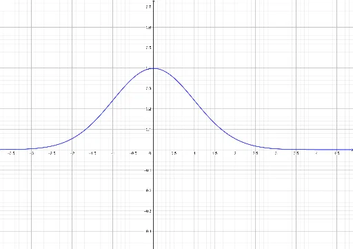
① This GeoGebra example dynamically illustrates the normal distribution probability density curve, showing how the mean μ and standard deviation σ affect the curve's position and shape. ② Core mathematical concepts include normal distribution, probability density function, symmetry, parameter effects, and the exponential function in the density formula. ③ Construction highlights: sliders g, μ, σ control parameters; parametric curves or function plotting are used to draw the bell curve; auxiliary shapes like rectangles or kites may visualize symmetry or area; object p likely represents a probability value or point. ④ Suitable for high school to college-level statistics teaching, ideal for classroom demonstrations of parameter changes, empirical rule, or student-driven exploration of distribution properties.
GeoGebra Commands & Parameters
g(x) = ℯ^(((-x^(2))) / 2) / ((abs(1) * sqrt((π * 2))))Numeric μ(0)1p(x) = ℯ^(((-(x - μ)^(2))) / ((2 * σ^(2)))) / sqrt(((2 * π) * σ^(2)))
AI Drawing Prompt Reference
Draw a dynamic normal distribution probability density curve that changes its position and shape by sliding μ and σ. First, plot a curve with the function e^(-1/2x^2). Then, add a slider for the mean μ, followed by a slider for the standard deviation σ. Finally, use parametric equations or a function to draw the normal distribution curve, and use auxiliary shapes to show symmetry or area.
The prompt above was compiled from the original drawing commands and is for reference only.