
Normal Distribution Demo by Cliff Packman
Loading the math board and drawing, please wait…
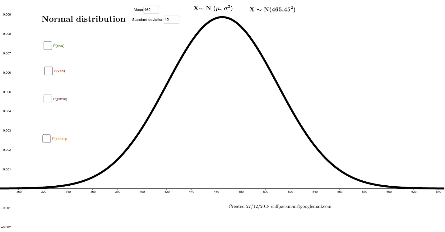
This example demonstrates the probability density function of the normal distribution and its properties. Key math concepts include normal distribution, differential calculus (integration, derivatives), and probability statistics. Construction highlights involve using commands like Normal for plotting, Textfield for text display, Integral for calculating integrals, and InverseNormal for inverse normal distribution calculations, with sliders to dynamically adjust parameters such as mean and standard deviation. Suitable for high school students and math enthusiasts learning probability and calculus.
GeoGebra Commands & Parameters
Normal(mean, stdev, x) → fTextfield(mean) → inputBox2Textfield(stdev) → inputBox3Textfield(a) → inputBox4Integral(f, -1.0E99, a) → bNormal(mean, stdev, a) → cIntegral(f, g, 1.0E99) → eTextfield(g) → inputBox1Textfield(j) → inputBox5Textfield(k) → inputBox6Integral(f, j, k) → mInverseNormal(mean, stdev, p) → oIntegral(f, -1.0E99, InverseNormal[mean, stdev, p]) → qTextfield(p) → inputBox7
AI Drawing Prompt Reference
Create a graph of the normal distribution probability density function with adjustable mean and standard deviation sliders. Show the integral area from negative infinity to a specified value and the integral result over a defined interval. Include the inverse normal distribution and probability calculations, all dynamically linked, suitable for students learning probability and calculus.
The prompt above was compiled from the original drawing commands and is for reference only.