
Normal Curve with Dynamic Standard Deviation
Loading the math board and drawing, please wait…
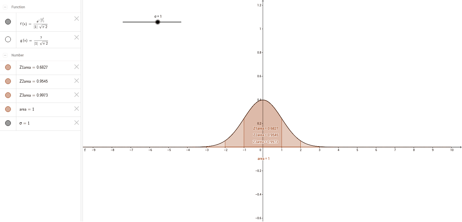
This example demonstrates how properties of the normal curve change when the standard deviation is altered. It involves core math concepts like normal distribution, standard deviation, and integral calculations. Constructed using GeoGebra commands Normal for the curve, Integral for area calculation, and a Slider to dynamically adjust σ. Key objects include f, c_1, g, c_2, area, Z1area, Z2area, Z3area. Suitable for high school and above, focusing on the impact of standard deviation on the shape and area of the normal distribution.
GeoGebra Commands & Parameters
Normal(0, σ, x) → fIntegral(f) → gIntegral(f, -10, 10) → areaIntegral(f, (-σ), σ) → Z1areaIntegral(f, (-2 * σ), (2 * σ)) → Z2areaIntegral(f, (-3 * σ), (3 * σ)) → Z3area
AI Drawing Prompt Reference
Draw a normal distribution curve with a dynamically adjustable standard deviation, including the integral area from -10 to 10 under the curve, and three dynamically changing integral areas based on the standard deviation σ: from -σ to σ, from -2σ to 2σ, and from -3σ to 3σ, with different colors or styles to show the impact of the standard deviation on the curve's shape and the areas.
The prompt above was compiled from the original drawing commands and is for reference only.