Normal Approximation to Binomial Distribution

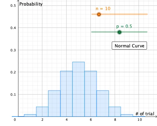
This GeoGebra example dynamically illustrates how the binomial probability histogram approaches the normal distribution curve as the number of trials n increases, demonstrating the central limit theorem in action. Core mathematical concepts include the binomial distribution, normal distribution, probability mass function vs. probability density function, and the approximation rule of thumb (np and n(1-p) both greater than 5). Construction details: the BinomialDist command generates the binomial probability histogram, the Normal command plots the corresponding normal curve with matching mean and standard deviation, sliders n and p adjust parameters, button1 triggers animation or toggles display, and a boolean variable controls the visibility of the normal approximation. Suitable for high school and college statistics courses, this interactive tool helps students grasp the central limit theorem and the conditions for normal approximation, and serves as a classroom demonstration or self-paced exploration resource.