
Non-Convex Robust PCA with Special Norm
Loading the math board and drawing, please wait…
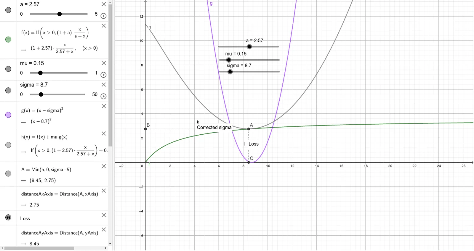
This example visualizes how a special norm works in non-convex robust PCA. It helps understand how special norms affect the results of PCA in non-convex optimization problems. Key mathematical concepts include non-convex optimization and robust PCA. GeoGebra commands used include Min, Midpoint, Distance, OrthogonalLine, Intersect, and Segment.
GeoGebra Commands & Parameters
Min(h, 0, (sigma * 5)) → AMidpoint(A, ClosestPoint[xAxis, A]) →Distance(A, xAxis) → distanceAxAxisMidpoint(A, ClosestPoint[xAxis, A]) →Distance(A, yAxis) → distanceAyAxisMidpoint(A, ClosestPoint[yAxis, A]) →OrthogonalLine(A, xAxis) → iOrthogonalLine(A, yAxis) → jIntersect(j, yAxis) → BSegment(A, B) → kIntersect(i, xAxis) → CSegment(A, C) → l
AI Drawing Prompt Reference
Draw the impact of a special norm in non-convex optimization. First, find the shortest distances from point A to the x-axis and y-axis, then construct the perpendicular lines from A to these axes, and finally connect point A to the intersection points B and C on the axes to form segments AB and AC.
The prompt above was compiled from the original drawing commands and is for reference only.