
Negative Binomial Distribution
Loading the math board and drawing, please wait…
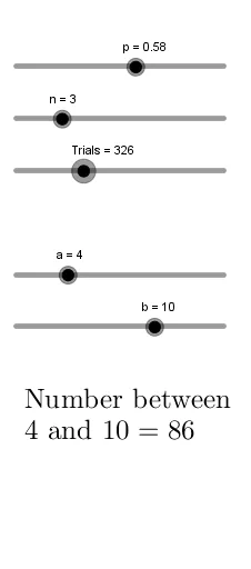
This example demonstrates the negative binomial distribution, a discrete probability distribution that models the number of trials needed to achieve a specified number of successes in a sequence of independent Bernoulli trials. By adjusting parameters n and p, the distribution's shape can be observed. The example uses commands like Sequence, Max, and CountIf, suitable for high school mathematics education and learning probability statistics.
GeoGebra Commands & Parameters
Sequence(Pascal[n, p, i, false], i, 1, 2000, 1) → probSequence(i, i, 1, 2000, 1) → numbersSequence(RandomDiscrete[numbers, prob], i, 1, t, 1) → list1Sequence(CountIf[x ≟ i, list1], i, 0, 2000, 1) → heightsSequence((i - 0.5, Element[heights, i + 1]), i, 0, 2000, 1) → Points1Sequence((i + 0.5, Element[heights, i + 1]), i, 0, 2000, 1) → Points2Max(Sequence[y(Element[Points1, i]), i, 1, Length[Points1]]) → hMax(Sequence[Element[list1, i], i, 1, Length[list1]]) → wCountIf(a ≤ x ∧ x ≤ b, list1) → cSequence(Polygon[(i - 0.5, 0), (i + 0.5, 0), Element[Points2, i + 1], Element[Points1, i + 1]], i, 0, 2000, 1) → list2