
Multivariate Limits Example 2
Loading the math board and drawing, please wait…
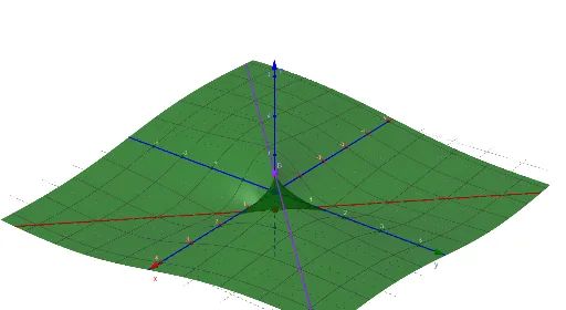
This example demonstrates the calculation and visualization of multivariate function limits. It involves core mathematical concepts such as multivariate limits, cubes, normal distributions, conic sections, ratios, and special points. The construction uses the GeoGebra command CurveCartesian with objects like f, a, A, b, c, B, C, d. Suitable for university-level mathematics or advanced calculus learners exploring multivariate limits.
GeoGebra Commands & Parameters
CurveCartesian(0, t, 0, t, -5, 5) → aCurveCartesian(t, 0, 0, t, -5, 5) → bCurveCartesian(t, t, 1 / 2, t, -5, 5) → cCurveCartesian(t, (-t), (-1) / 2, t, -5, 5) → d
AI Drawing Prompt Reference
Draw a 3D coordinate system illustrating a multivariate limit example. Include four straight-line paths in the coordinate plane: a vertical line along the y-axis from -5 to 5, a horizontal line along the x-axis from -5 to 5, a line with slope 1 passing through (0, 0.5), and a line with slope -1 passing through (0, -0.5). These paths approach the origin from different directions to show how function values vary. Clearly label the axes and emphasize the intersection of these paths near the origin to aid understanding of path dependence in multivariate limits.
The prompt above was compiled from the original drawing commands and is for reference only.