
Motion Detector
Loading the math board and drawing, please wait…
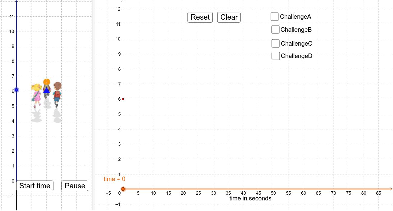
This example uses a motion detector to demonstrate function graphs and equations, helping students understand constant and variable rates of change. Key math concepts include functions, trigonometry, and piecewise functions. Construction involves GeoGebra commands like Function, time, ydistance, and sliders, suitable for high school mathematics teaching or self-learning.
GeoGebra Commands & Parameters
Function(6, 5, 7) → q_1Function((0 * x) + 6, 0, 10) → fFunction(((-0.5) * x) + 11, 10, 20) → gFunction((0.2 * x) - 3, 20, 40) → hFunction((0.1 * x) + 1, 40, 70) → pFunction(6, 0, 15) → t_1Function(((-0.05) * x) + 6.75, 15, 35) → rFunction(((-0.1) * x) + 8.5, 35, 55) → qFunction((-x) + 58, 55, 58) → sFunction(6, 0, 10) → g_1Function((3 * sin(((2 * π) * x / 40))) + 3, 10, 80) → f_1Function(6, 0, 10) → h_1Function((0.1 * x) + 5, 10, 30) → p_1Function(8, 30, 40) → r_1Function(((-0.5) * x) + 28, 40, 50) → s_1Function(((-0.3) * x) + 18, 50, 60) → t
AI Drawing Prompt Reference
Draw a motion detector example showing function graphs and equations, including constant and variable rates of change. Start by drawing a horizontal line y=6, then two lines with negative slopes, followed by two lines with positive slopes, and finally a sine curve y=3+3sin(πx/20). Connect all segments sequentially to form a dynamic graph.
The prompt above was compiled from the original drawing commands and is for reference only.