Monte Carlo random-sum stopping process to approximate Euler’s number e

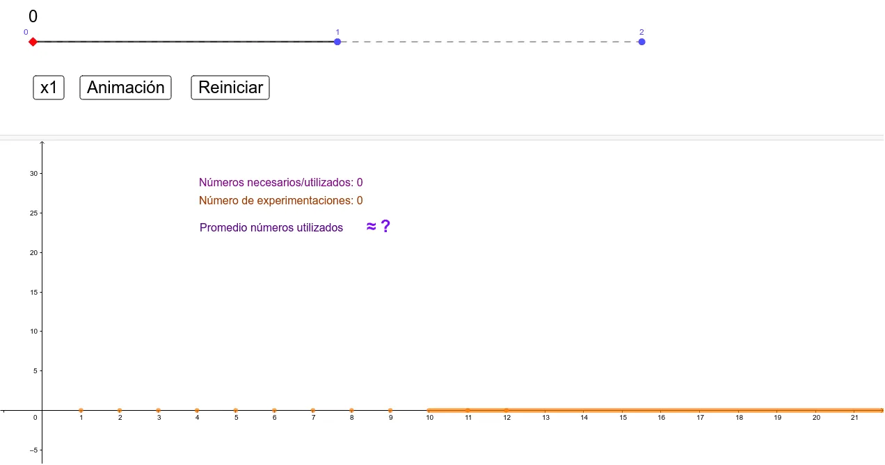
This example demonstrates a Monte Carlo stopping-time experiment: repeatedly choose numbers uniformly at random from 0 to 1, accumulate them step by step, and stop as soon as the running sum exceeds 1; then record how many draws were needed. By running (and visualizing) many trials, the construction illustrates a numerical approximation connection to Euler’s number e and the resulting distribution of stopping steps. The key math concepts are uniform random variables, first-passage/stop time, probability-statistics ideas (e.g., expectation/approximation via repeated sampling), and visualization of the empirical distribution such as boxplots. In GeoGebra, the build uses both geometric and logical components: Point and DynamicCoordinates to represent evolving states, Segment/Circle/Intersect to create auxiliary geometric references tied to the process, PolyLine to trace the progression, and If to implement the stopping rule when the accumulated result becomes greater than 1. LaTeX is used to label key quantities (threshold, counts, or derived parameters). The object structure (many sample variables and control/count symbols) supports aggregating repeated runs and displaying statistical summaries. Suitable for advanced high-school and introductory university courses in probability & statistics, and for interactive demonstrations of how randomized stopping processes produce approximations of e.