Matrix Transformations: Interactive Polygon Mapping

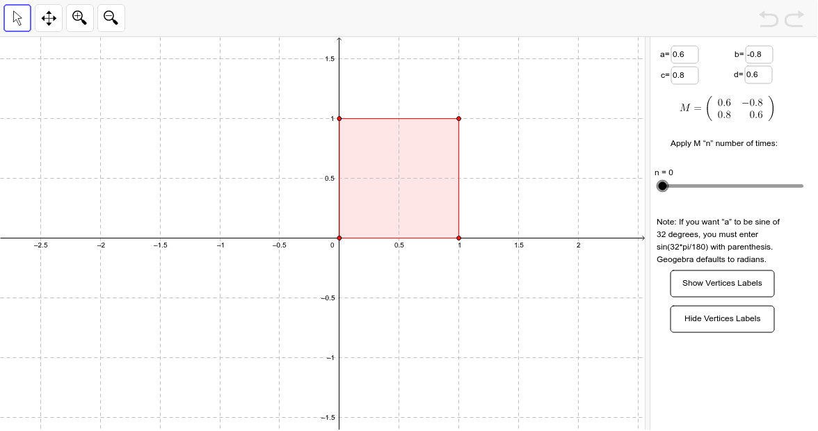
This GeoGebra example demonstrates how a polygon (e.g., a square) is transformed under a 2D linear transformation defined by a 2x2 matrix. Users can interactively edit the four matrix entries via input boxes, and instantly see the resulting image polygon, including effects like dilation, reflection, rotation, and shear. The core mathematical concepts are matrix multiplication, linear transformations, and their geometric interpretations (e.g., determinant affecting area scaling, sign indicating orientation). The construction uses GeoGebra commands: Polygon to create the original shape, ApplyMatrix to compute the transformed vertices, and Textfield/inputBox1-4 for dynamic matrix input. Additional objects like Intersect, Point, and text labels help visualize vertex correspondences. This resource is ideal for high school or introductory college linear algebra courses, enabling students to explore how different matrices (identity, diagonal, rotation, reflection) alter shapes, and to build intuition about eigenvectors, eigenvalues, and the geometric meaning of matrix operations.