
Mass, Volume, and Density Interactive Model
Loading the math board and drawing, please wait…
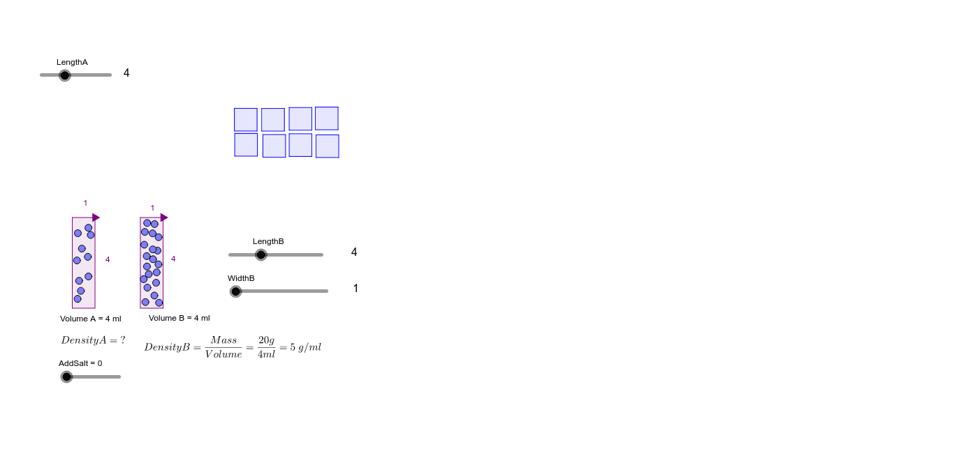
This GeoGebra example demonstrates how to understand density through an interactive rectangular prism model. Core mathematical concepts include the density formula ρ=m/v and the relationship between mass and volume. Construction details: Based on the construction summary, this model uses Polygon to draw rectangular prism faces, Point and Intersect to define vertices, OrthogonalLine to construct height; main objects include BoxA, BoxB (two adjustable prisms) and UnitVolume, with sliders or numeric inputs to change mass m and volume V, dynamically calculating and displaying density values. Suitable for middle school math or high school physics courses teaching density concepts.
GeoGebra Commands & Parameters
OrthogonalLine(A_1, xAxis) → aPoint(xAxis) → B_1OrthogonalLine(B_1, xAxis) → bOrthogonalLine(C, xAxis) → cOrthogonalLine(A_1, a) → dOrthogonalLine(C, b) → eIntersect(d, yAxis) → DIntersect(xAxis, yAxis) → EIntersect(a, xAxis) → FPolygon(A_1, D, E, F) → BoxA, a_1, d_1, e_1, fIntersect(c, xAxis) → GIntersect(b, e) → HPolygon(C, G, B_1, H) → BoxB, c_1, g, b_1, hPoint(Circle[I, 1]) → JPolygon(I, J, K, L) → UnitVolume, i, j, k, lPoint(Circle[I_1, 1]) → J_1Point(Circle[I_2, 1]) → J_2Point(Circle[I_3, 1]) → J_3Point(Circle[I_4, 1]) → J_4Point(Circle[I_5, 1]) → J_5Point(Circle[I_6, 1]) → J_6Point(Circle[I_7, 1]) → J_7PointIn(BoxA) → MPointIn(BoxA) → NPointIn(BoxA) → OPointIn(BoxA) → PPointIn(BoxA) → QPointIn(BoxA) → RPointIn(BoxA) → SPointIn(BoxA) → TPointIn(BoxA) → UPointIn(BoxA) → VPointIn(BoxB) → ZPointIn(BoxB) → C_1PointIn(BoxB) → D_1PointIn(BoxB) → E_1PointIn(BoxB) → F_1PointIn(BoxB) → G_1PointIn(BoxB) → H_1PointIn(BoxB) → M_1PointIn(BoxB) → N_1PointIn(BoxB) → O_1PointIn(BoxB) → P_1PointIn(BoxB) → Q_1PointIn(BoxB) → R_1PointIn(BoxB) → S_1PointIn(BoxB) → APointIn(BoxB) → BPointIn(BoxB) → T_1PointIn(BoxB) → U_1PointIn(BoxB) → V_1PointIn(BoxB) → W_1PointIn(BoxA) → WPointIn(BoxA) → Z_1PointIn(BoxA) → A_2PointIn(BoxA) → B_2PointIn(BoxA) → C_2PointIn(BoxA) → D_2PointIn(BoxA) → E_2PointIn(BoxA) → F_2PointIn(BoxA) → G_2PointIn(BoxA) → H_2Point(Circle[I_8, 1]) → J_8Point(Circle[I_9, 1]) → J_9Polygon(I_9, J_9, K_9, L_9) → UnitVolume_1, i_1, j_1, k_1, l_1Point(Circle[I_{10}, 1]) → J_{10}Polygon(I_{10}, J_{10}, K_{10}, L_{10}) → UnitVolume_2, i_2, j_2, k_2, l_2Point(Circle[I_{11}, 1]) → J_{11}Polygon(I_{11}, J_{11}, K_{11}, L_{11}) → UnitVolume_3, i_3, j_3, k_3, l_3Point(Circle[I_{12}, 1]) → J_{12}Polygon(I_{12}, J_{12}, K_{12}, L_{12}) → UnitVolume_4, i_4, j_4, k_4, l_4Point(Circle[I_{13}, 1]) → J_{13}Polygon(I_{13}, J_{13}, K_{13}, L_{13}) → UnitVolume_5, i_5, j_5, k_5, l_5Point(Circle[I_{14}, 1]) → J_{14}Polygon(I_{14}, J_{14}, K_{14}, L_{14}) → UnitVolume_6, i_6, j_6, k_6, l_6Point(Circle[I_{15}, 1]) → J_{15}Polygon(I_{15}, J_{15}, K_{15}, L_{15}) → UnitVolume_7, i_7, j_7, k_7, l_7
AI Drawing Prompt Reference
Please draw an interactive rectangular prism model to understand the concept of density. The model includes two adjustable rectangular prisms, BoxA and BoxB, and a unit volume rectangular prism, UnitVolume. Use sliders or numeric inputs to change mass m and volume V, dynamically calculating and displaying density values. Main objects include the faces, vertices, and height lines of the prisms. Construction sequence: First, draw the faces of the prisms, then define the vertices and height lines, and finally add sliders or numeric inputs to adjust mass and volume.
The prompt above was compiled from the original drawing commands and is for reference only.