
Mapping Diagram of Complex Derivative for Power Functions
Loading the math board and drawing, please wait…
In collections
Mapping Diagrams to Visualize Complex Analysis
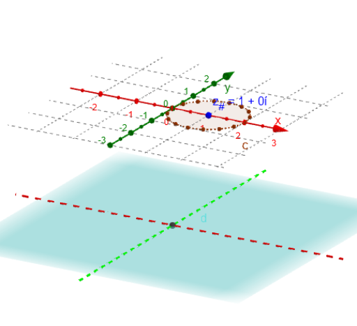
① This example visualizes the mapping diagram of the derivative of complex power functions f(z)=z^n, showing how each input point maps to its derivative output. ② Core mathematical concepts: complex numbers, complex functions, derivatives, power functions, mapping diagrams, local linearization. ③ Construction highlights: Derivative computes the derivative; Sequence and Zip create a grid of sample points; Circle, Line, Vector, and Point draw input and output vectors; Locus tracks the mapping trajectories; Textfield displays the exponent n and error estimates. ④ Suitable for university complex analysis courses, advanced calculus instruction, and research visualization.
GeoGebra Commands & Parameters
Derivative(g) → dgSequence(0, m) → MZip(((2 * π) * k / m), k, M) → t_*Zip((δ * ℯ^((t * ί))) + z_#, t, t_*) → z_*Circle(z_#, δ) → cLine(O, ZY1) → YaxLine(O, ZX1) → XaxVector(z_#, Gz1_#) → vecg_#Point(c) → ALocus(PtAG, A) → gLocZip(g(z), z, z_*) → gz_*Zip((x(z), y(z), ht), z, gz_*) → gpt_*Zip(Vector[A, B], A, z_*, B, gpt_*) → gvec_*Zip(z - z_#, z, z_*) → dz_*Zip((dG_# * z), z, dz_*) → dG_*Zip(gz_# + w, w, dG_*) → Estgz_*Zip((x(z), y(z), ht), z, Estgz_*) → Estgpt_*Zip(Vector[A, B], A, z_*, B, Estgpt_*) → Estgvec_*Zip(dg(z), z, z_*) → Dgz_*Zip((x(z), y(z), ht), z, Dgz_*) → Dgpt_*Zip(Vector[A, B], A, z_*, B, Dgpt_*) → Dgvec_*Derivative(G1, z) → dG1Textfield(G1) → InputBox1
AI Drawing Prompt Reference
Create a mapping diagram for the derivative of complex power functions f(z)=z^n, showing how input points map to their derivative outputs. Generate a grid of sample points, compute their derivatives, and draw vectors for inputs and outputs. Include input points, output vectors, and mapping trajectories, with the exponent n and error estimates displayed. Connect trajectories with points and represent errors with vectors to visualize the local linearization of the function.
The prompt above was compiled from the original drawing commands and is for reference only.