
Mapping Diagram for Newton's Method in Complex Analysis
Loading the math board and drawing, please wait…
In collections
Mapping Diagrams to Visualize Complex Analysis
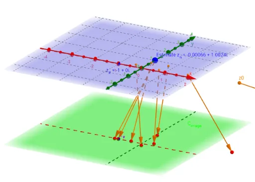
This example demonstrates the mapping process and iterative trajectories of Newton's method in the complex plane. It involves core mathematical concepts such as complex numbers, derivatives, iterative functions, and mapping relationships. The construction utilizes GeoGebra commands and objects like Element, Derivative, Sequence, Zip, If, CurveCartesian, Textfield, Vector, Integral, Point, Locus, IterationList, Iteration, etc. It is suitable for teaching and demonstrating complex analysis, numerical methods, and advanced mathematics.
GeoGebra Commands & Parameters
Element(zfnlist, n_f) → FDerivative(g) → g'Sequence(t, t, t_0, t_2, dt) → t_*Element(xfnlist, n_γ) → x_γElement(yfnlist, n_γ) → y_γZip(x_γ(B) + (y_γ(B) * ί) + z_#, B, t_*) → z_*Sequence(t, t, t_0 + dt, t_2 + dt, dt) → t_1Zip(x_γ(B) + (y_γ(B) * ί) + z_#, B, t_1) → z_1Zip(t - u, t, z_1, u, z_*) → dz_*If(Align ≟ 1, z_# - fz_#, 0) → alignSequence(((Element[fz_*, k] - align) * Element[dz_*, k]), k, 1, n) → fdz_*Sequence(Sum[fdz_*, k], k, 1, n) → SUMfdz_*Zip((x(B), y(B), ht), B, fz_*) → fpoint_*Zip((x(Z) + x(align), y(Z) + y(align), ht), Z, SUMfdz_*) → ESumSequence(Element[dz_*, k], k, 1, n) → dz_nCurveCartesian(x_γ(t) + x(z_#), y_γ(t) + y(z_#), t, t_0, t_2) → γTextfield(x_γ) → inputxtTextfield(y_γ) → inputytVector(z_#, Pfz_#) → uTextfield(F) → InputFzZip(Vector[A, B], A, z_*, B, fpoint_*) → fvec_*Integral(f) → Int_fElement(z_*, 1) → z_0Element(z_*, n + 1) → z_2Point(γ) → AγLocus(FAγ3, Aγ) → fLocZip(Vector[A, B], A, z_*, B, ESum) → ESumV_*CurveCartesian(t + x(align), y(align), ht, t, -5, 5) → XhCurveCartesian(x(align), t + y(align), ht, t, -5, 5) → YhIterationList(Newton(z), z, {z0}, n_N) → NewtlistZip((x(A), y(A), ht), A, fnewtlist) → ptfnewtlistZip(Vector[A, B], A, Newtlist, B, ptfnewtlist) → vecnewtlistIteration(Newton(z), z, {z0}, n_N) → Newtest
AI Drawing Prompt Reference
Draw a mapping diagram for Newton's method in the complex plane, showing iterative trajectories. Start by plotting the mapping relationship of the function with curves, marking initial and final points. Then, represent directional changes with vectors and draw the accumulated effect of trajectories. Finally, display the iteration process, distinguishing each step's trajectory with different colors, and label key points and function values.
The prompt above was compiled from the original drawing commands and is for reference only.