
Mapping Diagram for Cauchy Integral Formula
Loading the math board and drawing, please wait…
In collections
Mapping Diagrams to Visualize Complex Analysis
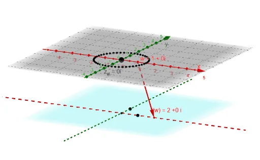
This example demonstrates the mapping diagram of the Cauchy Integral Formula, visually illustrating the properties of complex function integration through dynamic graphics. Core mathematical concepts include complex functions, integration, mapping, and complex number operations. The construction leverages GeoGebra commands and objects like Sequence, Zip, Circle, Line, Vector, Point, Locus, ToComplex, and Textfield to build function mappings and integral paths. It is suitable for university mathematics students or learners of complex function theory, providing an intuitive understanding of abstract integral concepts.
GeoGebra Commands & Parameters
Sequence(0, n) → NZip(((2 * pi) * k / n), k, N) → t_*Zip((r * ℯ^((t * ί))) + z_#, t, t_*) → z_*Circle(z_#, r) → cZip(f_I(z), z, z_*) → fz_*Zip((x(z), y(z), ht), z, fz_*) → fpt_*Line(O, ZS1) → YaxLine(O, ZR1) → XaxZip(Vector[A, B], A, z_*, B, fpt_*) → gvec_*Vector(z_#, fz1_#) → vecf_#Point(c) → ALocus(PtfA, A) → fLocSequence(Element[z_*, k + 1] - Element[z_*, k], k, 1, n) → dzSequence((Element[fz_*, k] * Element[dz, k]), k, 1, n) → fdz_*Sequence((1 / (((2 * pi) * ί)) * Sum[fdz_*, k]), k, 1, n) → Sumfdz_*ToComplex(Sum[fdz_*, n]) → EstIntZip(ToComplex[A], A, Sumfdz_*) → SumComx_*Zip((x(A), y(A), ht), A, SumComx_*) → Sumfdz3_*Zip(Vector[A, B], A, z_*, B, Sumfdz3_*) → SumVec_*Textfield(F) → InputBox1Vector((x(w), y(w)), Ptfw) → vecfw
AI Drawing Prompt Reference
Create a mapping diagram for the Cauchy Integral Formula, showing a circle and its internal mapped complex function curves, integral paths, and function value changes, demonstrating the properties of complex function integration through dynamic graphics. Key elements include a circle, mapped curves, integral paths, and function value points, with construction starting from the base circle and axes, followed by mapping curves and integral paths, and ending with labeled function value points and integral results.
The prompt above was compiled from the original drawing commands and is for reference only.