
Make Histogram: Dynamic Data Distribution Visualization
Loading the math board and drawing, please wait…
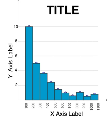
① This example demonstrates how to dynamically construct a histogram in GeoGebra to visualize data distribution, allowing users to adjust parameters and observe changes in the graph. ② Core mathematical concepts include data grouping, frequency counting, histograms and frequency distributions, with extensions to linear programming, logarithms, parabolas, fractal geometry, and subtraction. ③ Construction highlights: based on the summary, it uses GeoGebra commands such as Point, OrthogonalLine, Polygon, and RotateText, involving objects A through U, V, W, Z, and subscripted points. Rectangular bars are drawn using polygons, perpendicular lines assist positioning, and rotated text labels annotations. ④ Suitable for middle school statistics and probability lessons, as well as introductory college data analysis, helping learners understand data visualization and distribution characteristics.
GeoGebra Commands & Parameters
Point(xAxis) → APoint(xAxis) → BPoint(xAxis) → CPoint(xAxis) → DPoint(xAxis) → EPoint(xAxis) → FPoint(xAxis) → GPoint(xAxis) → HPoint(xAxis) → IPoint(xAxis) → JPoint(xAxis) → KPoint(xAxis) → LPoint(xAxis) → MPoint(xAxis) → NPoint(xAxis) → OPoint(xAxis) → PPoint(xAxis) → QPoint(xAxis) → RPoint(xAxis) → SPoint(xAxis) → TPoint(xAxis) → UOrthogonalLine(L, xAxis) → fOrthogonalLine(M, xAxis) → gOrthogonalLine(N, xAxis) → hOrthogonalLine(O, xAxis) → iOrthogonalLine(P, xAxis) → jOrthogonalLine(Q, xAxis) → kOrthogonalLine(R, xAxis) → lOrthogonalLine(S, xAxis) → mOrthogonalLine(T, xAxis) → nOrthogonalLine(U, xAxis) → pPoint(f) → VPoint(g) → WPoint(h) → ZPoint(i) → A_1Point(j) → B_1Point(k) → C_1Point(l) → D_1Point(m) → E_1Point(n) → F_1Point(p) → G_1OrthogonalLine(V, yAxis) → qOrthogonalLine(W, yAxis) → rOrthogonalLine(Z, yAxis) → sOrthogonalLine(A_1, yAxis) → tOrthogonalLine(B_1, yAxis) → aOrthogonalLine(C_1, yAxis) → bOrthogonalLine(D_1, yAxis) → cOrthogonalLine(E_1, yAxis) → dOrthogonalLine(F_1, yAxis) → eOrthogonalLine(G_1, yAxis) → f_1Point(q) → H_1Point(q) → I_1Point(r) → J_1Point(r) → K_1Point(s) → L_1Point(s) → M_1Point(t) → N_1Point(t) → O_1Point(a) → P_1Point(a) → Q_1Point(b) → R_1Point(b) → S_1Point(c) → T_1Point(c) → U_1Point(d) → V_1Point(d) → W_1Point(e) → Z_1Point(e) → A_2Point(f_1) → B_2Point(f_1) → C_2Polygon(B, I_1, H_1, A) → q1, b_1, i_1, h_1, a_1Polygon(B, J_1, K_1, C) → q2, b_2, j_1, k_1, c_1Polygon(D, M_1, L_1, C) → q3, d_1, m_1, l_1, c_2Polygon(D, E, O_1, N_1) → q4, d_2, e_1, o_1, n_1Polygon(E, F, Q_1, P_1) → q5, e_2, f_2, q_1, p_1Polygon(F, G, S_1, R_1) → q6, f_3, g_1, s_1, r_1Polygon(G, H, U_1, T_1) → q7, g_2, h_2, u_1, t_1Polygon(H, I, W_1, V_1) → q8, h_3, i_2, w_1, v_1Polygon(I, J, A_2, Z_1) → q9, i_3, j_2, a_2, z_1Polygon(J, K, C_2, B_2) → q10, j_3, k_2, l_2, m_2RotateText("100", 90°) → text1RotateText("200", 90°) → text1_1RotateText("300", 90°) → text1_{10}RotateText("400", 90°) → text1_2RotateText("500", 90°) → text1_3RotateText("600", 90°) → text1_4RotateText("700", 90°) → text1_5RotateText("800", 90°) → text1_6RotateText("900", 90°) → text1_7RotateText("1000", 90°) → text1_8RotateText("1100", 90°) → text1_9RotateText("Y Axis Label", 90°) → text3