
Logarithmic Gravitational Field Model
Loading the math board and drawing, please wait…
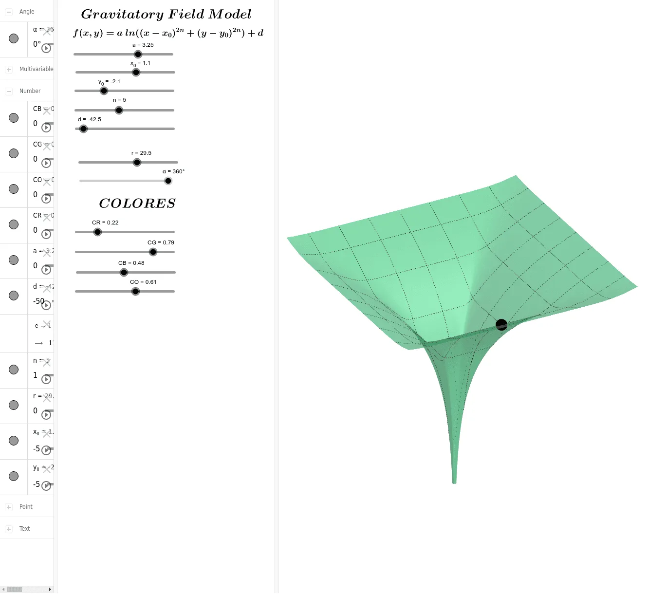
This example demonstrates the graphical representation and physical significance of a logarithmic gravitational field model. Key mathematical concepts include logarithmic functions, coordinate geometry, and vector operations. Construction highlights involve GeoGebra commands and objects such as a, CR, CG, CB, CO, x_0, y_0, n, d, fm, texto1, texto2, texto3, r, α, e, A for parametric modeling and dynamic visualization. Suitable for high school students and enthusiasts in physics and mathematics to understand gravitational field distribution and logarithmic function applications.
GeoGebra Commands & Parameters
Numeric a(3.25)Numeric CR(0.22)Numeric CG(0.79)Numeric CB(0.48)Numeric CO(0.61)Numeric x_0(1.1)Numeric y_0(-2.1)Numeric n(5)Numeric d(-42.5)fm(x, y) = ((1 / 2 * a) * log((x - x_0)^((2 * n)) + (y - y_0)^((2 * n)))) + dNumeric r(29.5)Angle α(6.283185307179586)((1 / 2 * a) * log(((r * cos(α)) - x_0)^((2 * n)) + ((r * sin(α)) - y_0)^((2 * n)))) + d(x_0 + (r * cos(α)), y_0 + (r * sin(α)), fm(x_0 + (r * cos(α)), y_0 + (r * sin(α))))
AI Drawing Prompt Reference
Draw a logarithmic gravitational field model. The model includes parameters a, x_0, y_0, n, d, r, and α, along with the function fm. The construction order is: first define these parameters, then define the function fm, then calculate the point (x_0 + r*cos(α), y_0 + r*sin(α)), and finally compute the gravitational field value at that point. The graph illustrates the distribution of the gravitational field, demonstrating the application of logarithmic functions in physics.
The prompt above was compiled from the original drawing commands and is for reference only.