
Logarithmic Function Practice: Graph Properties and Transformations
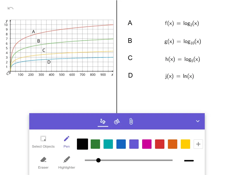
Loading the math board and drawing, please wait…
This example demonstrates how logarithmic functions behave on the coordinate plane, focusing on their characteristic graph features and how the curve changes under common transformations. You can observe the domain restrictions, the vertical asymptote at x=0, monotonic behavior (depending on the base a), and how the overall shape is controlled by parameter changes. The key math concepts are the definition and properties of logarithmic functions y=log_a(x), including base-related effects on increasing/decreasing trends and the geometric meaning of key points. In GeoGebra, the construction is typically done by defining the function expression to generate the graph, then using transformation tools (e.g., shifts and dilations) to map a standard log graph to the target one, while optionally adding reference lines such as the asymptote or axes to read geometric relationships. Suitable for high-school (and pre-AP/contest) students as well as guided classroom practice on function graphing.
AI Drawing Prompt Reference
Draw the graph of a logarithmic function y = log_a(x) on a coordinate plane, emphasizing its key behaviors: the domain restriction x > 0 and a vertical asymptote at x = 0 showing the curve cannot cross that line. Choose the base a to reflect the characteristic monotonic trend (increasing for some bases, decreasing for others) and to demonstrate how changing parameters alters the overall shape. Include the coordinate axes as reference and optionally annotate a few key geometric points to support reading positions on the graph. Construct by first generating a standard log curve from the function definition, then apply shifts and dilations to map it to the intended target form while keeping the asymptote and axes aligned.
The prompt above was compiled from the original drawing commands and is for reference only.