
Logarithmic Function Graph Transformation
Loading the math board and drawing, please wait…
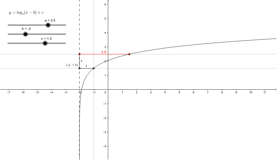
This example demonstrates how adjusting parameters a, b, and c in the equation y = log_a(x-b) + c affects the graph of the logarithmic function. Key mathematical concepts include properties of logarithmic functions, the impact of parameters on graph shape, and coordinate transformations. Construction involves GeoGebra commands such as Intersect, OrthogonalLine, Circle, and Segment. Suitable for middle or high school mathematics learning to understand logarithmic function graph transformations and practical applications.
GeoGebra Commands & Parameters
Intersect(f, e, (-1, 1.5)) → AOrthogonalLine(A, e) → gIntersect(g, yAxis) → BIntersect(d, g) → CCircle(C, A) → hIntersect(h, d) → D, EOrthogonalLine(D, d) → iIntersect(f, i, (1.4999999997916815, 2.499999999952489)) → FIntersect(d, xAxis) → GIntersect(d, g) → HIntersect(d, i) → IIntersect(f, i, (1.4999999997916815, 2.499999999952489)) → JIntersect(e, g) → KSegment(I, J) → jSegment(H, K) → kSegment(I, H) → l
AI Drawing Prompt Reference
Draw a logarithmic function graph and show how adjusting parameters a, b, and c changes its shape. Start by plotting the logarithmic function, then find intersections with the x and y axes. Construct perpendicular lines and a circle using these points. Identify intersections of the circle with the function graph and draw line segments between these points to visualize the transformation process.
The prompt above was compiled from the original drawing commands and is for reference only.