
Lissajous Curves with Equilateral Triangles
Loading the math board and drawing, please wait…
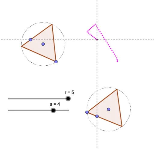
This example demonstrates how to construct Lissajous curves using equilateral triangles, illustrating the geometric relationship between parametric equations and loci. Key math concepts include the symmetry of equilateral triangles, the application of trigonometric functions, parametric equation plotting, and locus generation. Construction highlights involve GeoGebra commands/objects like Point, Circle, Polygon, OrthogonalLine, and Intersect. Suitable for high school mathematics education, emphasizing the integration of parametric equations, loci, and geometric transformations.
GeoGebra Commands & Parameters
Point(yAxis) → ACircle(A, 1) → cPoint(xAxis) → BCircle(B, 1) → dPoint(d) → CPoint(c) → DPolygon(C, Rotate[C, (2 * π / 3), B], 3) → poly1, f, g, h, EPolygon(D, Rotate[D, (2 * π / 3), A], 3) → poly2, i, j, k, FPoint(poly1) → GPoint(poly2) → HOrthogonalLine(H, yAxis) → lOrthogonalLine(G, xAxis) → mIntersect(l, m) → I