
Linear Regression of Student Scores
Loading the math board and drawing, please wait…
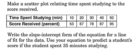
This GeoGebra example demonstrates how to perform a linear regression on a set of student score data, visually showing the scatter plot and the best-fit line. The core mathematical concepts include linear regression, least squares method, the equation of the fitted line, the geometric meaning of slope and intercept, and statistical distribution of data points. Construction highlights: the FitLineY command generates the regression line, Point and Segment mark data points and connecting segments, Slope and Intersect compute the line's slope and intersections, mean calculates averages, and TableText displays the data table. Multiple text objects (text1 to text9) annotate key values and the equation. Suitable for high school or college statistics and data analysis courses, this example helps students understand how regression models describe linear relationships between variables and how to assess the fit quality.
GeoGebra Commands & Parameters
FitLineY({A, B, C, D, E}) → aIntersect(yAxis, a) → GSlope(a) → mPoint(a) → JPoint(a) → KLine(J, xAxis) → bLine(K, yAxis) → cIntersect(b, c) → LSegment(J, L) → dSegment(L, K) → emean(B2:B6) → y_mmean(B7:B7) → gTableText({{A1, B1, C1, D1, E1, F1, G1}, {A2, B2, C2, D2, E2, F2, G2}, {A3, B3, C3, D3, E3, F3, G3}, {A4, B4, C4, D4, E4, F4, G4}, {A5, B5, C5, D5, E5, F5, G5}, {A6, B6, C6, D6, E6, F6, G6}, {A7, B7, C7, D7, E7, F7, G7}}, "|_") → text12
AI Drawing Prompt Reference
Create a coordinate-plane scatter plot using the provided student score data points. Add the best-fit line obtained by a least-squares linear regression through those points, and mark the intersections between the fitted line and the coordinate axes. Highlight the key points on the fitted line used for describing the regression, and draw connecting line segments between those points and the axis intersection to emphasize the geometric relationships. Compute the mean value(s) from the relevant data column(s) and include an on-figure data table/text area summarizing the dataset together with the computed regression-related values. Add annotations for the fitted line’s slope and intercept-related information.
The prompt above was compiled from the original drawing commands and is for reference only.