Lagrange Optimization Demonstration

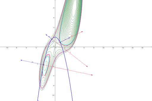
This example illustrates the geometric meaning of the Lagrange multiplier method in three-dimensional space by dynamically adjusting parameters to observe the maximum and minimum values of the objective function under constraints. Key mathematical concepts include Lagrange multipliers, geometric mean, statistics, trigonometric functions, and 3D surfaces. Construction highlights involve using the Vector command to build vectors, f_x, f_y for partial derivatives, list1 for data points, and a as a parameter, with objects like LL, D, E, F, c, H, e, d, Y, g, J, h, B, A, u, v, w, i, j, k, l, m, p, n, o, q for 3D graph construction and calculations. Suitable for university students and researchers in mathematics, physics, and engineering studying optimization methods.