Kepler's Laws of Planetary Motion

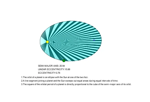
This example dynamically demonstrates Kepler's three laws of planetary motion, visually illustrating the elliptical orbit of planets around a star, the constant areal velocity, and the direct proportionality between the square of the orbital period and the cube of the semi-major axis. Core mathematical concepts include ellipses, vectors, coordinate geometry, and integral calculus for area calculation and limit concepts. GeoGebra commands like ellipse construction, rotation, line, intersection, vector, tangent, orthogonal line, midpoint, and parameters are used to simulate planetary motion trajectories and velocity changes. Suitable for high school students and above, or enthusiasts studying celestial mechanics and analytical geometry as a teaching or research tool.