
IS-PC-MR Model with Anchored Expectations
Loading the math board and drawing, please wait…
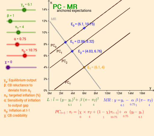
This example demonstrates the IS-PC-MR model with anchored expectations. Key mathematical concepts include equations, logarithmic functions, means, and statistical characteristics. Using GeoGebra commands such as IntersectPath, Point, Intersect, and Tangent, complex mathematical graphics are constructed. Suitable for high school and above mathematics education and research.
GeoGebra Commands & Parameters
IntersectPath(xOyPlane, l) → l_oPoint(l_o) → E_TIntersect(PC_0, pis, (6.1, 10.75)) → E_0Tangent(g_a, c) → g_b, g_cIntersect(c, g_b, 1) → AIntersect(h, xAxis) → CIntersect(PC_0, MR, (2.8600000000000003, 8.32)) → E_sIntersect(MR, PC_1, (2.86, 8.32)) → E_1Intersect(g_e, h) → E_2Point(MR) → EIntersect(MR, g_f, (4.772895999999999, 5.769472)) → E_3Intersect(MR, g_h, (5.25065344, 5.13246208)) → E_4Intersect(MR, g_i, (5.5564182016, 4.7247757312)) → E_5Intersect(IS, w_0, (6.1, 3.4800000000000013)) → R_0Intersect(IS, w_1, (2.86, 5.856000000000001)) → R_1Intersect(IS, w_2, (4.0264, 5.000640000000001)) → R_2Intersect(IS, w_3, (4.772895999999999, 4.453209600000001)) → R_3Intersect(IS, w_4, (5.25065344, 4.102854144000001)) → R_4Intersect(IS, w_5, (5.5564182016, 3.8786266521600012)) → R_5Intersect(IS, w_T, (6.1, 3.4800000000000013)) → R_T
AI Drawing Prompt Reference
Draw a macroeconomic diagram with IS, PC (two curves PC_0 and PC_1), and MR curves. Mark the initial equilibrium, target equilibrium, and several intermediate adjustment points, which are intersections of PC with MR, and IS with vertical lines representing different expectations. Include tangent lines from the initial point, and a horizontal line (anchored expectation) intersecting the PC curve. Label all key points with solid dots, use smooth curves, and clearly show axes.
The prompt above was compiled from the original drawing commands and is for reference only.