
Inverse Cosine Function
Loading the math board and drawing, please wait…
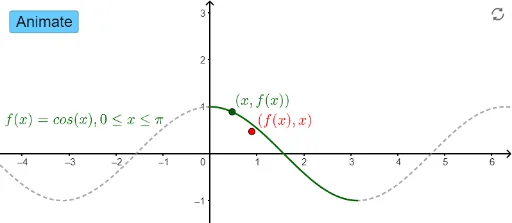
This example demonstrates the graph and properties of the inverse cosine function. It involves core math concepts like inverse trigonometric functions, cosine function, and coordinate geometry. Constructed using GeoGebra commands such as CurveCartesian, Point, and Mirror. Suitable for high school mathematics teaching to understand the domain, range, and graph characteristics of the inverse cosine function.
GeoGebra Commands & Parameters
CurveCartesian((t, f(t)), t, 0, π) → aPoint(a) → AMirror(A, y = x) → A'Mirror(a, y = x) → f_1
AI Drawing Prompt Reference
Draw the graph of the inverse cosine function. Start by plotting the cosine curve for x from 0 to π as the original function. Then pick an arbitrary point on this curve and reflect it across the line y = x. Next, reflect the entire cosine curve across the same line to obtain the inverse cosine graph. The final image should include the original cosine curve, its reflected curve, the chosen point and its reflection, and the line y = x as the axis of symmetry, illustrating the domain, range, and shape of the inverse cosine function.
The prompt above was compiled from the original drawing commands and is for reference only.