Intersections of Polynomial Functions: Dynamic Exploration

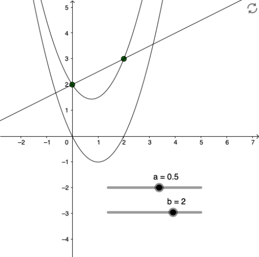
①This GeoGebra example dynamically demonstrates the intersection points of two polynomial functions, visually showing where their function values are equal and the corresponding x- and y-coordinates. ②Core mathematical concepts include polynomial functions, solving equations, intersection points of graphs, and the idea of combining algebra with geometry. ③Construction highlights: from the summary, objects f, a, b, g, h, and list1 are used; f and g are polynomial functions, a and b may be parameters or x-coordinates of intersections, h may be an auxiliary function or line, and list1 stores the list of intersection coordinates, computed dynamically via commands. ④Suitable for middle and high school mathematics (from upper middle school to high school) when learning functions and equations, as well as for pre-college review, helping students understand the geometric meaning of polynomial equation roots and fostering dynamic exploration and visual analysis skills.