
Interactive Visualization of Hypothesis Testing Using the Binomial Distribution
Loading the math board and drawing, please wait…
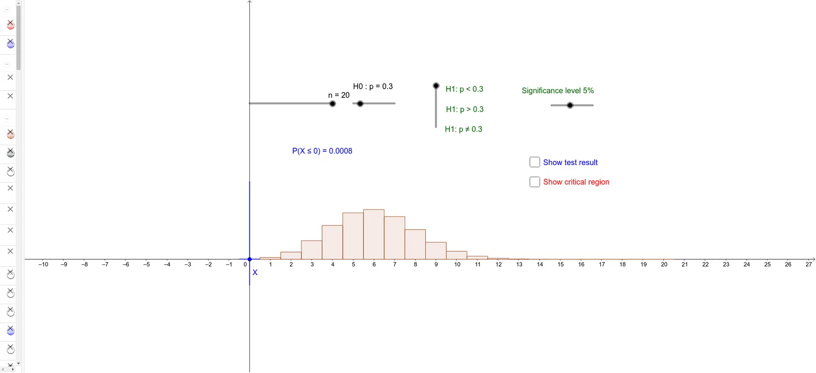
This GeoGebra example demonstrates hypothesis testing based on the binomial distribution through an interactive visualization. It shows the probability mass function under the null hypothesis, highlights the rejection region, and marks the critical values and the observed test statistic. Core mathematical concepts include binomial distribution, hypothesis testing, significance level, critical region, and p-value. The construction uses commands such as Sequence to generate binomial probabilities, BarChart to plot the distribution, Element to extract specific values, Segment and Point to delineate the rejection region and test statistic, along with sliders for parameters like p and n to dynamically update the graph and textual outputs. Suitable for high school and introductory college statistics courses, this example helps learners grasp the decision-making process of hypothesis testing and visualize how the rejection boundary shifts with sample size and significance level.
GeoGebra Commands & Parameters
Sequence(((nCr[n, r] * p^(r)) * (1 - p)^(n - r)), r, 0, n) → LBarChart(-0.5, n + 0.5, L) → aSequence(Sum[L, i], i, 1, n + 1) → SBarChart(-0.5, c_1 + 0.5, Take[L, 1, c_1 + 1]) → cBarChart(c_2 - 0.5, n + 0.5, Take[L, c_2 + 1, n + 1]) → dBarChart(-0.5, c_3 + 0.5, Take[L, 1, c_3 + 1]) → fElement(S, c_3 + 1) → s_3BarChart(c_4 - 0.5, n + 0.5, Take[L, c_4 + 1, n + 1]) → gSegment(A, B) → iPoint(i) → XSegment((x(X), 0.3), (x(X), -0.1)) → jBarChart(-0.5, x(X) + 0.5, Take[L, 1, x(X) + 1]) → kElement(S, x(X) + 1) → x_1BarChart(x(X) - 0.5, n + 0.5, Take[L, x(X) + 1, n + 1]) → lElement(S, c_1 + 1) → s_1
AI Drawing Prompt Reference
Create an interactive visualization showing hypothesis testing based on the binomial distribution. Include a bar chart for the probability mass function under the null hypothesis, highlight the rejection region with different colors or shading, and mark critical values and the observed test statistic. Use sliders to dynamically change parameters p and n, observing the changes in the distribution, rejection boundary, and test statistic.
The prompt above was compiled from the original drawing commands and is for reference only.