Hydraulic System Curve: Interactive Pipe Resistance and Pump Operating Point

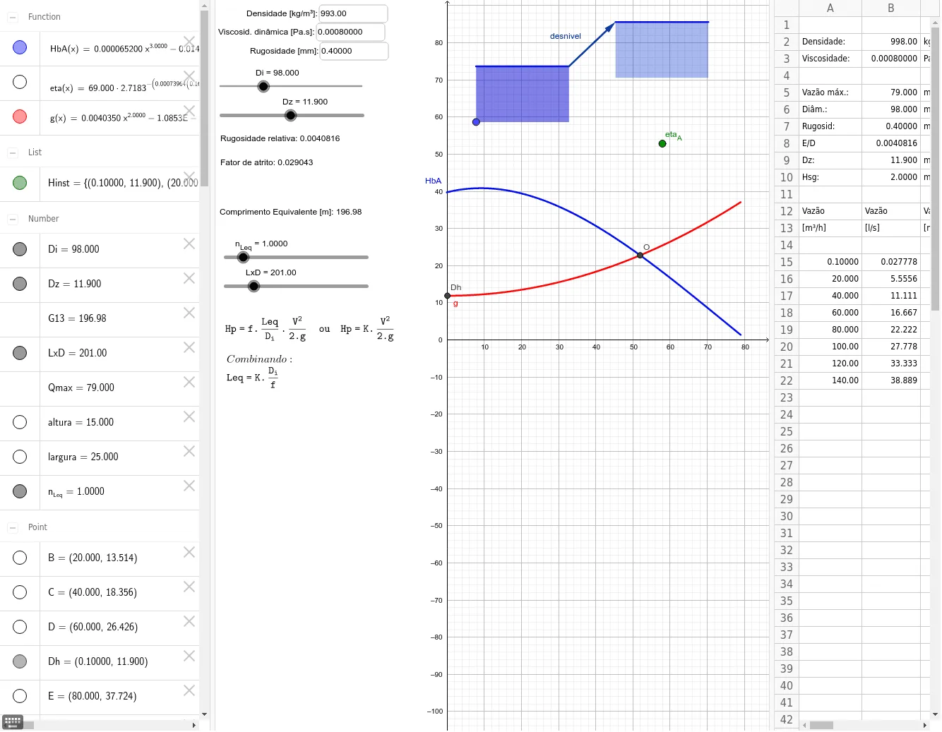
This GeoGebra example demonstrates the construction of a hydraulic system curve, showing how the required head (altura) varies with flow rate (Q) in a pipe network. The core mathematical concepts involve quadratic functions (head loss proportional to flow squared), piecewise functions for different flow regimes, and the intersection of curves to determine the pump operating point. The construction uses GeoGebra commands such as Textfield for parameter input, If for conditional logic, Intersect to find the crossing of pump and system curves, Polygon to shade regions, Vector to indicate flow direction, and Point to mark key locations. Key objects include n_Leq (equivalent length), LxD (length-diameter product), Di (inner diameter), Qmax (maximum flow), altura (head), and numerous auxiliary points (A12~A22, B12~B22, C12~C22) that define the curve geometry and labels. This resource is suitable for high school to university-level courses in fluid mechanics, engineering hydraulics, or applied mathematics, helping students visualize how changing pipe parameters shifts the system curve and affects the operating point. It also serves as an excellent example of parametric modeling and interactive graphing in STEM education.