
Histogram with Unequal Class Intervals
Loading the math board and drawing, please wait…
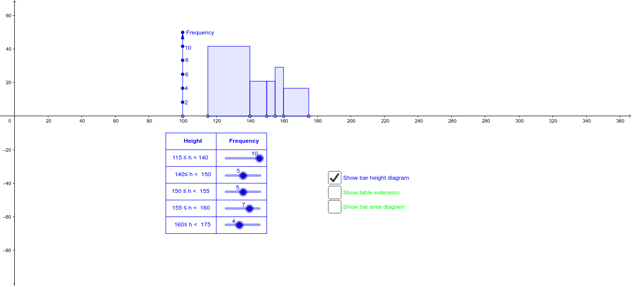
This GeoGebra example demonstrates how to create a histogram with unequal class intervals. Unlike equal-width histograms, the height of each bar in an unequal-interval histogram represents frequency density (frequency divided by class width), which accurately reflects the data distribution. Key mathematical concepts include frequency density, class width, and frequency distribution. Construction uses Sequence to generate multiple bars of varying widths, Point/Line/Segment to define bar vertices, Polygon to form closed bar regions, and lists to manage data. Suitable for secondary school statistics teaching and university-level probability courses.
GeoGebra Commands & Parameters
OrthogonalLine(S, y = 0) → l_1Point(l_1) → ZPoint(xAxis) → APoint(xAxis) → BLine(A, B) → k_1Point(xAxis) → CPoint(xAxis) → DPoint(xAxis) → EPoint(xAxis) → FSequence((x(G), y(G) - (10 * i)), i, 1, 6) → liste1Sequence((x(H), y(H) - (10 * i)), i, 1, 6) → liste2Sequence((x(I), y(I) - (10 * i)), i, 1, 6) → liste3Sequence((x(J), y(J) - (10 * i)), i, 1, 6) → liste4Sequence((x(K), y(K) - (10 * i)), i, 1, 6) → liste5Point(liste1) → LSegment(G, L) → aPoint(liste2) → MSegment(H, M) → bPoint(liste3) → NSegment(I, N) → cPoint(liste4) → OSegment(J, O) → dPoint(liste5) → PSegment(K, P) → eSequence(Segment[(x(G), y(G) - (10 * i)), (x(G) + 60, y(G) - (10 * i))], i, 0, 6) → liste6Sequence(Segment[(x(G) + 90, y(G) - (10 * i)), (x(G) + 60, y(G) - (10 * i))], i, 0, 6) → liste7Vector(S, Z) → uPolygon(A, B, (x(B), ((f * 0.1) * y(V))), (x(A), ((f * 0.1) * y(V)))) → poly1, p, q, r, sPolygon(B, C, (x(C), ((g * 0.1) * y(V))), (x(B), ((g * 0.1) * y(V)))) → poly2, t, a_1, b_1, c_1Polygon(C, D, (x(D), ((h * 0.1) * y(V))), (x(C), ((h * 0.1) * y(V)))) → poly3, d_1, e_1, f_1, m_1Polygon(D, E, (x(E), ((i * 0.1) * y(V))), (x(D), ((i * 0.1) * y(V)))) → poly4, g_1, h_1, n_1, p_1Polygon(E, F, (x(F), ((j * 0.1) * y(V))), (x(E), ((j * 0.1) * y(V)))) → poly5, i_1, j_1, q_1, r_1Point(l_1) → WVector(S, W) → vPolygon(A, B, (x(B), (h1 * y(E_1))), (x(A), (h1 * y(E_1)))) → poly6, s_1, t_1, a_2, b_2Polygon(B, C, (x(C), (h2 * y(E_1))), (x(B), (h2 * y(E_1)))) → poly7, b_3, c_2, d_2, e_2Polygon(C, D, (x(D), (h3 * y(E_1))), (x(C), (h3 * y(E_1)))) → poly8, c_3, d_3, f_2, g_2Polygon(D, E, (x(E), (h4 * y(E_1))), (x(D), (h4 * y(E_1)))) → poly9, d_4, e_3, h_2, i_2Polygon(E, F, (x(F), (h5 * y(E_1))), (x(E), (h5 * y(E_1)))) → poly10, e_4, f_3, j_2, k_2
AI Drawing Prompt Reference
Draw a histogram with unequal class intervals on a coordinate plane. Place six points sequentially on the x-axis to define five intervals of varying widths. For each interval, construct a rectangle whose base is the interval and whose height equals the frequency divided by the class width, representing frequency density. Use polygons to form five closed rectangular bars with different widths but heights calculated precisely from frequency density values. The area of each bar accurately reflects the frequency distribution. The resulting statistical histogram is suitable for teaching probability and data distribution concepts.
The prompt above was compiled from the original drawing commands and is for reference only.