
Hessian Matrices and Quadratic Forms
Loading the math board and drawing, please wait…
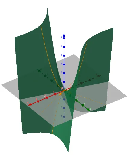
This example illustrates the relationship between Hessian matrices and quadratic forms. Key concepts include quadratic forms, Hessian matrices, eigenvalues, and eigenvectors. Using GeoGebra commands such as Root, If, UnitVector, etc., the example constructs the graph of a quadratic form and analyzes its properties. Suitable for college-level mathematics and linear algebra courses.
GeoGebra Commands & Parameters
Root(((a - x) * (c - x)) - b^(2)) → R_2, R_1If(b ≟ 0, (1, 0), ((-b), a - λ_1)) → EigUnitVector(Vector[Eig]) → v_1UnitOrthogonalVector(v_1) → v_2Line((0, 0), N_2) → l_1Line((0, 0), N_1) → l_2Line((0, 0), v_1) → E_1Line((0, 0), v_2) → E_2CurveCartesian(((v_1 * i) * t), ((v_1 * e_2) * t), f(((v_1 * i) * t), ((v_1 * e_2) * t)), t, -3, 3) → eCurveCartesian(((v_2 * i) * t), ((v_2 * e_2) * t), f(((v_2 * i) * t), ((v_2 * e_2) * t)), t, -3, 3) → g
AI Drawing Prompt Reference
Draw a graph of a quadratic form defined by a symmetric matrix with entries a, b, and c. First, compute the eigenvalues of the matrix and determine the corresponding eigenvectors. From the origin, draw two lines along these eigenvector directions to represent the principal axes. Also draw two lines orthogonal to these eigenvectors. Then, for each eigenvector direction, plot a three-dimensional curve parameterized by t from -3 to 3, where the height is given by the quadratic form function evaluated along that direction. The final figure shows the cross-sections of the quadratic surface along the eigenvector directions, along with the eigenvector and orthogonal lines.
The prompt above was compiled from the original drawing commands and is for reference only.