
Hand-Made Best Fit Lines
Loading the math board and drawing, please wait…
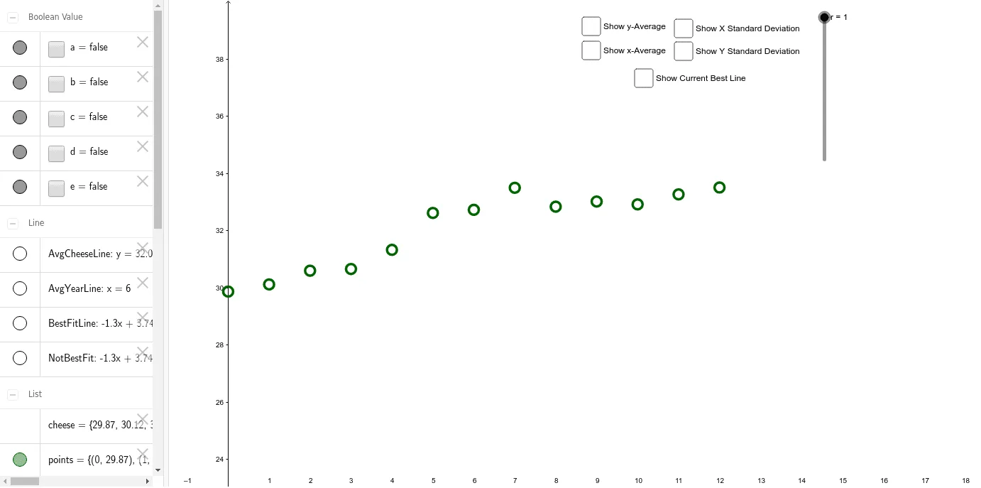
This example demonstrates how to draw best fit lines manually, illustrating linear regression concepts. Key mathematical concepts include linear regression, correlation, and geometric construction. Construction involves GeoGebra commands like Zip, SD, Mean, Segment, and Line to calculate standard deviation, mean, and fitted lines. Suitable for high school students or college students for learning statistics and geometry, useful in teaching or self-study.
GeoGebra Commands & Parameters
Zip((r, c), c, cheese, r, years) → pointsSD(years) → SD_{years}SD(cheese) → SD_{cheese}Mean(cheese) → AVG_{cheese}Mean(years) → AVG_{year}Segment(A, (x(B), y(A))) → SdYearLineSegment(B, (x(B), y(A))) → SdCheeseLineLine(A, C) → BestFitLineLine(A, B) → NotBestFitSegment(C, (x(B), y(A))) → rSD_{cheese}
AI Drawing Prompt Reference
Draw a graph showing best fit lines. Include scatter points, a best fit line, and a non-best fit line. The best fit line should represent the trend of the data points, while the non-best fit line serves as a comparison. The graph should clearly illustrate linear regression concepts to help understand data distribution and fitting methods.
The prompt above was compiled from the original drawing commands and is for reference only.