
Half-Life Action (3)!!! Dynamic Illustration of Half-Life Independence from Init
Loading the math board and drawing, please wait…
In collections
Exploring Exponential & Logarithmic Functions
Exploring Exponential & Logarithmic Functions
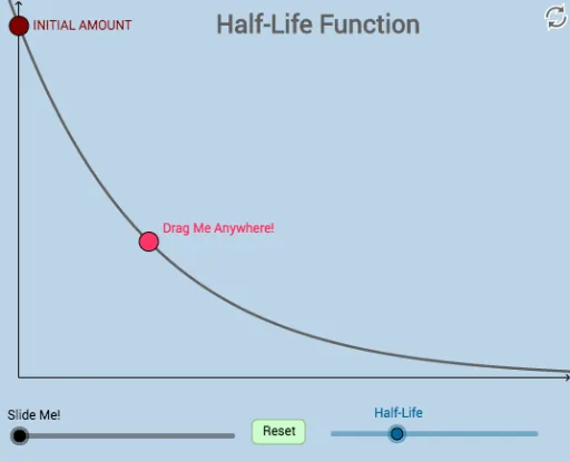
① This dynamic GeoGebra example demonstrates that the half-life of a decaying substance is independent of its initial amount, using adjustable parameters and interactive visuals. ② Core mathematical concepts include exponential decay, half-life, proportionality, function graphs, and transformations such as translation and scaling. ③ Construction highlights: based on the summary, it employs text fields (Textfield/InputBox) for initial amount a_0 and decay constant k, along with commands like Intersect, Midpoint, Dilate, Rotate, Translate, Integral, Ray, Point, Vector, and Segment to build a modifiable illustration with multiple geometric objects and input boxes. ④ Suitable for high school physics or mathematics classes exploring exponential functions and half-life, as well as introductory college courses or STEM outreach, emphasizing the scale-invariant nature of half-life.
GeoGebra Commands & Parameters
Textfield(a_0) → InputBox1Textfield(k) → InputBox2Intersect(A, b, (315.1, 600)) → DIntersect(A, c, (630.2, 300)) → EIntersect(A, d, (945.3000000000001, 150)) → FIntersect(A, e, (1260.4000000000003, 74.99999999999994)) → GTextfield(f) → InputBox3Intersect(b, h) → HSegment(H, D) → iIntersect(c, j) → IIntersect(d, l) → JSegment(I, E) → mSegment(J, F) → nSegment(D, I) → pSegment(E, J) → qIntersect(h, s) → KIntersect(r, t) → LSegment(K, C) → f_1Segment(C, L) → g_1Midpoint(M, Initial) → NDilate(M, If[0 < o ≤ 1, 1 - o, 0], N) → M'Rotate(M, If[1 < o ≤ 2, ((o - 1) * π), π], N) → M'_1Rotate(M', If[1 < o ≤ 2, ((o - 1) * π), π], N) → M''Dilate(N, If[2 < o ≤ 3, 3 - o, 0], D) → N'Segment(N, N') → j_1Dilate(Initial, If[0 < o ≤ 1, 1 - o, 0], N) → B'Segment(Initial, B') → h_1Rotate(Initial, If[1 < o ≤ 2, ((-(o - 1)) * π), (-π)], N) → B'_1Rotate(B', If[1 < o ≤ 2, ((-(o - 1)) * π), (-π)], N) → B''Segment(B'_1, B'') → i_1Rotate(N', If[6 < o ≤ 7, ((-(o - 6)) * π), (-π)], D) → N''Integral(A, 0, Infinity) → o_1Ray((0, 0), (1, 0)) → g_2Textfield(u_1) → InputBox4Textfield(val) → InputBox5Point(A) → RIntersect(k_1, y = 0) → SMidpoint(R, S) → UIntersect(A, l_1, (747.0739488341455, 231.98826691092705)) → WDilate(R, If[3 < o ≤ 4, 4 - o, 0], U) → R'Segment(R, R') → m_1Dilate(U, If[4 < o ≤ 5, 5 - o, 0], S) → U'Segment(U, U') → n_1Rotate(R, If[5 < o ≤ 6, ((-(o - 5)) * π), (-π)], U) → R'_1Rotate(R', If[5 < o ≤ 6, ((-(o - 5)) * π), (-π)], U) → R''Segment(R'_1, R'') → p_1Dilate(U, If[6 < o ≤ 7, 7 - o, 0], W) → U'_1Segment(U, U'_1) → t_1Dilate(N, If[7 < o ≤ 8, 8 - o, 0], U) → N'_1Vector(N, N'_1) → uTranslate(N, u) → N'_2Translate(N', u) → N''_1Segment(N'_2, N''_1) → a_1
AI Drawing Prompt Reference
Draw a dynamic illustration showing that half-life is independent of initial amount. Include an exponential decay curve with two input boxes to adjust the initial amount and decay constant. Mark several equally spaced time points on the curve, and drop perpendiculars to the time axis to form rectangles representing the amount lost in each half-life. Use dashed lines to indicate the half-life levelscars, and connect the initial point to these time points. Add a slider to animate the process of halving, rotating, or scaling, and show the integral area for total decay. Include axes, grid, and labels for clarity.
The prompt above was compiled from the original drawing commands and is for reference only.