Graphing Secant Line to Approximate the Derivative

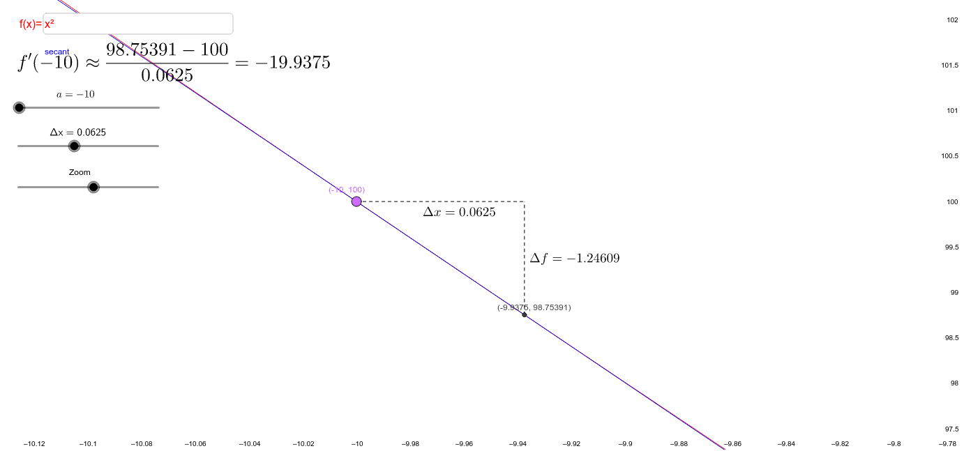
This example demonstrates how to approximate the derivative of a function at a point using a secant line. Core math concepts include derivatives, secant lines, function graphs, and linear approximation. It utilizes GeoGebra commands like Segment, Line, Textfield, Point, and objects such as a, SecondPoint, dx, f, f2, f1, P, A, Δx, P_2, Δf, slope, secant, Zoom, text2, text3, text4, text1, inputBox1, df, text5, B, C, text6, ymin2, ymax, xmax, xmin for construction. Suitable for high school and above students learning calculus to understand the geometric meaning of derivatives and the secant line approximation method.