
Graphing Quadratic Equations by RobArbonTuition
Loading the math board and drawing, please wait…
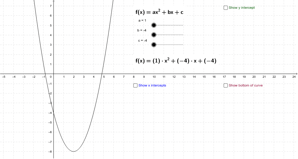
This example demonstrates how the graph of a quadratic function changes with varying coefficients, visually showing the effects on x and y intercepts and the vertex of the parabola. Key math concepts include quadratic functions, coefficient influence, intercept calculations, and vertex coordinates. It utilizes GeoGebra objects like a, b, c, x_1, x_2, A, C, xone, xtwo, d, p, q, e, g, text4, text2, f, text2_1, q_1, text3, text1. Suitable for A*-B level iGCSE students to understand quadratic function properties and coefficient effects.
GeoGebra Commands & Parameters
Numeric a(1.0)Numeric b(-4.0)Numeric c(-4.0)((-b + sqrt(b^(2) - 4 * a * c)) / (2 * a), 0)((-b - sqrt(b^(2) - 4 * a * c)) / (2 * a), 0)((-b) / (2 * a), (-b^(2)) / (4 * a) + c)(0, c)x(x_1)x(x_2)Boolean d(false)x(A)y(A)Boolean e(false)Boolean g(false)f(x) = a * x^(2) + b * x + cb^(2) / (4 * a)
AI Drawing Prompt Reference
Draw the graph of a quadratic function, showing how changes in coefficients affect the shape, including x and y intercepts and the vertex. Adjust the coefficients a, b, c to see the graph transform, and label the x-intercepts, vertex, and y-intercept with their coordinates. Use distinct colors or styles for key points and add text annotations for their coordinate values.
The prompt above was compiled from the original drawing commands and is for reference only.