
Graphing Linear Equations in 2 Unknowns with Circumcircle and Scatter Plot
Loading the math board and drawing, please wait…
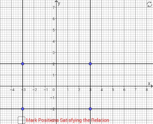
This GeoGebra example demonstrates how to graph linear equations in two unknowns, showing straight lines along with a circumcircle, scatter plot, and elements of linear programming. The core mathematical concepts include linear equations, straight lines, circumscribed circles, scatter plots, and linear optimization. Construction uses the Sequence and Line commands, involving objects such as S, T, U, V, int, list1 through list4, A, text1, b, c, text3, A1, B1, C1, texto1, D1, f, g, B, h, and i. These commands generate multiple lines and associated geometric elements, with text labels for clarity. Suitable for middle and high school students learning about graphing linear equations, line properties, and introductory linear programming, as well as for teachers demonstrating these concepts interactively.
GeoGebra Commands & Parameters
Sequence(Segment[(x(S) + (int * i), y(S)), (x(T) + (int * i), y(T))], i, 0, (x(U) - x(T)) / int) → list1Sequence(Segment[(x(T), y(T) + (int * i)), (x(U), y(U) + (int * i))], i, 0, (y(S) - y(T)) / int) → list2Sequence(Segment[(x(S) + (int * i / 5), y(S)), (x(T) + (int * i / 5), y(T))], i, 0, (5 * (x(U) - x(T)) / int)) → list3Sequence(Segment[(x(T), y(T) + (int * i / 5)), (x(U), y(U) + (int * i / 5))], i, 0, (5 * (y(S) - y(T)) / int)) → list4Line(A1, B1) → fLine(B1, C1) → gLine(B, C1) → hLine(B, A1) → i