
Graphing Exponential Functions -01
Loading the math board and drawing, please wait…
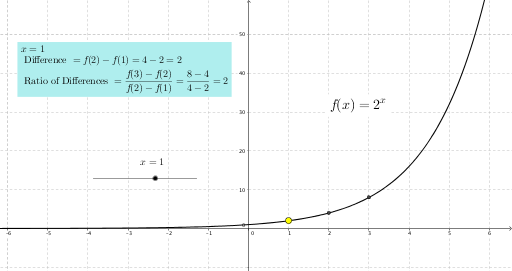
This example demonstrates how to graph exponential functions using GeoGebra and explore the differences and ratios of differences. Key math concepts include exponential function properties, difference analysis, and function graphing. GeoGebra commands used: f (exponential function), x_p (point), A, C, B (parameters), xa, xb, xc, ya, yb, yc (data points), diff (difference), rdiff (ratio of difference), text2, text1, text3 (text annotations). Suitable for high school mathematics teaching to understand exponential growth characteristics and data analysis.
GeoGebra Commands & Parameters
f(x) = 2^(x)Numeric x_p(1.0)(x_p, f(x_p))(x_p + 2, f(x_p + 2))(x_p + 1, f(x_p + 1))x(A)x(B)x(C)y(A)y(B)y(C)yb - ya(yc - yb) / (yb - ya)
AI Drawing Prompt Reference
Plot the exponential function y=2^x and mark a point at x=1. Then, mark two additional points to the right of this point at intervals of 1 and 2 units, and connect them. Add three parameter points, label their x and y coordinates. Finally, calculate and display the difference between two y-coordinates and the ratio of these differences to illustrate exponential growth characteristics and difference analysis.
The prompt above was compiled from the original drawing commands and is for reference only.