Graphical Solution of a Linear Programming Maximization Problem

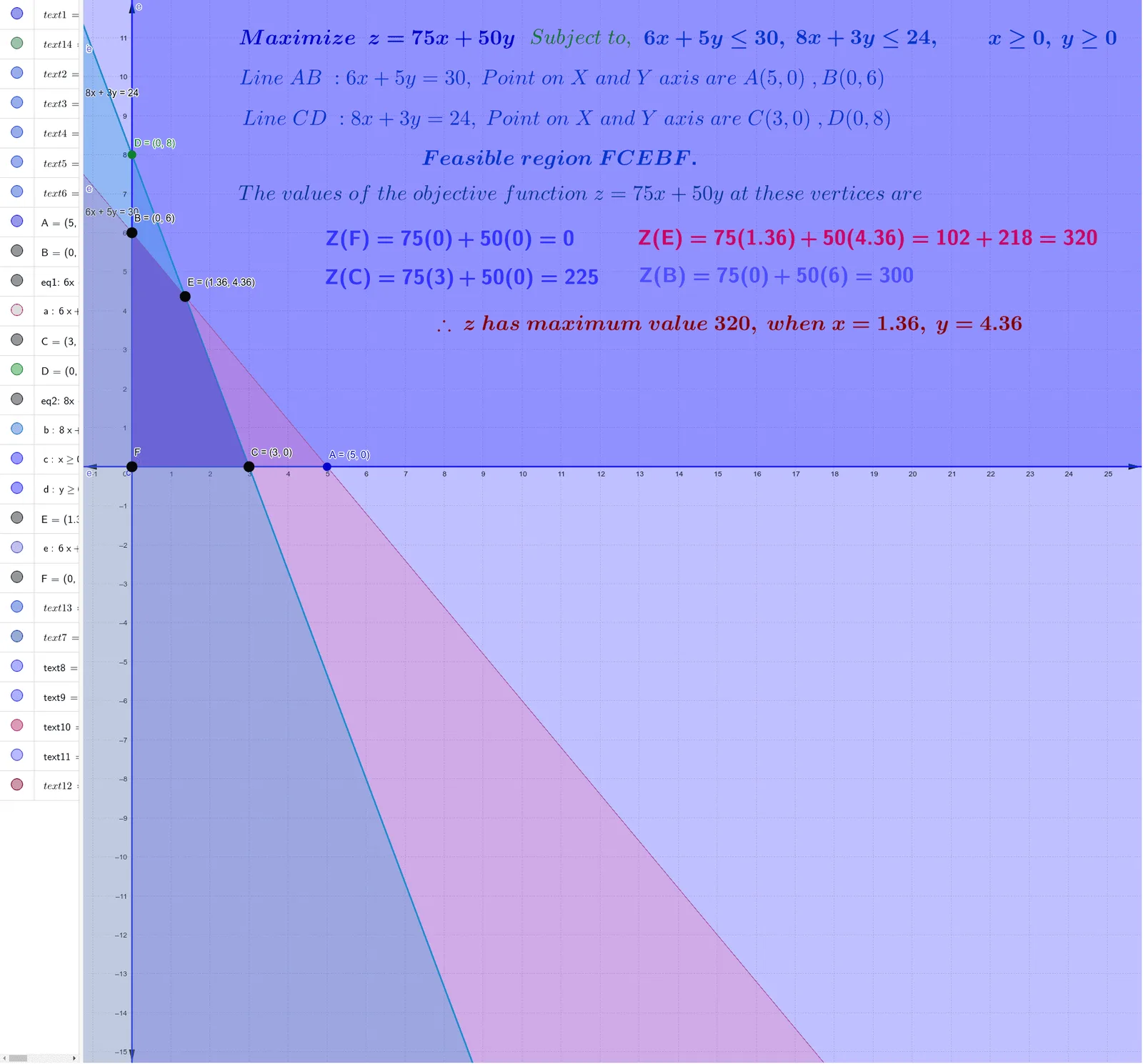
This example demonstrates how to solve a linear programming maximization problem using the graphical method: it visualizes the feasible region and shows how the optimum for the objective function is determined from the geometry of that region. Key concepts include linear programming/linear optimization, linear constraints and the resulting feasible set, and maximizing a linear objective via geometric reasoning (the optimum occurs at a vertex/intersection point under typical conditions). In construction, the workflow is built around GeoGebra commands Point and Intersect: Point is used to create and label key candidate points (such as A–F and related labeled vertices), while Intersect computes the intersection points of constraint lines to obtain the feasible-region corners. Additional equation and text objects (e.g., eq1/eq2 and multiple text labels) organize the constraints and the objective-function presentation so learners can directly read off the optimal solution from the constructed graph. Suitable for high school through early university courses in optimization, operations research, and graphing-based understanding of inequalities and linear functions.