
Graphical and Numerical Solution of Nonlinear Systems by Roman Chijner
Loading the math board and drawing, please wait…
In collections
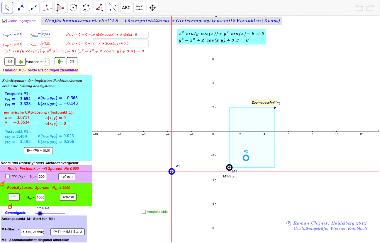
Solution of Systems of nonlinear Equations
This example demonstrates the graphical and numerical solution of a system of two nonlinear equations in two variables, incorporating zoom functionality to explore local solutions. Key math concepts include nonlinear systems, graphical methods, numerical computation, and zoom operations. GeoGebra commands and objects used in construction are Corner, Defined, Ray, Point, If, Locus, Textfield, Polygon, Sequence, RemoveUndefined, Join, Text, Intersect. Suitable for high school and above students to understand nonlinear equation solving and graphical representation.
GeoGebra Commands & Parameters
Corner(2, 5) → Co5Defined(Co5) → aM3Ray(M1, Vector[Corner[2, 5]]) → M32Point(M32) → M3rIf(aM3, M3r, B) → M3Point(Segment[Px2, Px1]) → AxPoint(Segment[Py2, Py1]) → AyIf(Funktion ≟ 1, a(x, y), If[Funktion ≟ 2, b(x, y), a(x, y) * b(x, y)]) → f00If((f1(x0 - ε / 2) * f1(x0 + ε / 2) < 1.0E-8) ∧ (f2(x0 - ε / 2) * f2(x0 + ε / 2) < 1.0E-8), (x0, y0)) → E0xIf((g1(y0 - ε / 2) * g1(y0 + ε / 2) < 0) ∧ (g2(y0 - ε / 2) * g2(y0 + ε / 2) < 0), (x0, y0)) → E0yIf(fxx(xi - ε / 2) * fxx(xi + ε / 2) < 0, (xi, y(Ay))) → Bxx1If(fyy(yi - ε / 2) * fyy(yi + ε / 2) < 0, (x(Ax), yi)) → Byy1Locus(Bxx1, Ay) → locxx1Locus(Byy1, Ax) → locyy1Textfield(a) → inputBox1Textfield(b) → inputBox2Polygon((x_{max}, y_{max}), (x_{min}, y_{max}), (x_{min}, y_{min}), (x_{max}, y_{min})) → VV, d, e, g, hTextfield(N_P) → Textfeld1If(a_1, N_P, 2) → N_1Sequence(x_{min} + (x_{max} - x_{min}) / N_1 * i, i, 0, N_1) → xxSequence(y_{min} + (y_{max} - y_{min}) / N_1 * i, i, 0, N_1) → yyRemoveUndefined(Join[Zip[Mirror[{Roots[f00(a, x), y_{min}, y_{max}]}, y = x] + (a, 0), a, xx]]) → PxxyJoin(Zip[Reverse[{Roots[f00(x, b), x_{min}, x_{max}]}] + (0, b), b, yy]) → PyyxTextfield(Funktion) → Textfeld2Textfield(x_{min}) → Textfeld3Textfield(y_{min}) → Textfeld4Textfield(x_{max}) → Textfeld5Textfield(y_{max}) → Textfeld6Textfield(N) → Textfeld7Text(Element[L, 1]) → LxText(Element[L, 2]) → LyTextfield(M10) → Textfeld8Intersect(Element[L, 1], Element[L, 2]) → C
AI Drawing Prompt Reference
Create an interactive graph for solving a system of two nonlinear equations. The view shows two editable input boxes for the functions. On the coordinate plane, plot two curves representing the equations, with a grid for reference. Include draggable points to set initial guesses. Display two locus curves tracing the roots in the x and y directions, and mark the intersection point as the numerical solution. Provide text fields for adjusting the x and y ranges, grid density, and iteration count, plus a button to trigger computation. At the intersection of the two curves, show a distinct point with its coordinates labeled.
The prompt above was compiled from the original drawing commands and is for reference only.