
Geometric Surface Fitting and Optimization
Loading the math board and drawing, please wait…
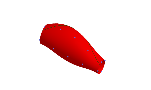
This example demonstrates how to construct a surface using polynomial fitting and involves optimization problems. Key mathematical concepts include function fitting, optimization methods, and probability distributions. Construction involves GeoGebra commands such as Point, FitPoly, and Surface. Suitable for high school or university mathematics courses to learn geometric modeling and optimization techniques.
GeoGebra Commands & Parameters
Point(yAxis) → CPoint(yAxis) → C'Point(x = 1) → DPoint(x = 1) → D'Point(x = -2) → APoint(x = -2) → A'Point(x = -1) → BPoint(x = -1) → B'Point(x = 2) → EPoint(x = 2) → E'FitPoly({C, D, A, B, E}, 4) → fy1FitPoly({C', D', A', B', E'}, 4) → fy2Line((-2, my(-2), 0), zAxis) → dz1Line((-1, my(-1), 0), zAxis) → dz2Line((0, my(0), 0), zAxis) → dz3Line((1, my(1), 0), zAxis) → dz4Line((2, my(2), 0), zAxis) → dz5Point(dz1) → FPoint(dz1) → F'Point(dz2) → GPoint(dz2) → G'Point(dz3) → HPoint(dz3) → H'Point(dz4) → IPoint(dz4) → I'Point(dz5) → JPoint(dz5) → J'Sequence((x(Element[Lz3d, i]), z(Element[Lz3d, i])), i, 1, 5) → LzSequence((x(Element[Lzz3d, i]), z(Element[Lzz3d, i])), i, 1, 5) → LzzFitPoly(Lz, 4) → fz1FitPoly(Lzz, 4) → fz2Surface(u, my(u) + (ry(u) * cos(v)), mz(u) + (rz(u) * sin(v)), u, -2, 2, v, -3.14159, 3.141592653589793) → aSequence(CurveCartesian[t, my(t) + (ry(t) * cos(t + i)), mz(t) + (rz(t) * sin(t + i)), t, -2, 2], i, 0, (2 * π) - (2 * π / n), (2 * π / n)) → liste1Sequence(CurveCartesian[t, my(t) + (ry(t) * cos((-t) + i)), mz(t) + (rz(t) * sin((-t) + i)), t, -2, 2], i, 0, (2 * π) - (2 * π / n), (2 * π / n)) → liste2
AI Drawing Prompt Reference
Create a 3D surface defined by two 4th-degree polynomial functions fz1 and fz2. The surface intersects with a series of lines dz1 to dz5 parallel to the z-axis at points F to J, which are then used to fit the surface.
The prompt above was compiled from the original drawing commands and is for reference only.