Geometric Sensitivity Analysis for Linear Programming

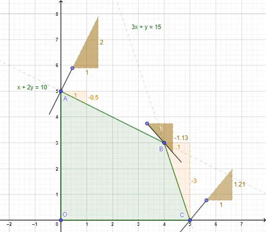
This example demonstrates—via geometry—how the optimal solution of a linear programming (LP) problem changes when the objective function coefficients vary, and how to identify the region of parameter values for which the same vertex remains optimal. It builds the feasible region as a polygon and relates optimality to geometric conditions between objective-direction lines (level sets) and the polygon’s edges/vertices. Key concepts include linear programming, feasible polytope geometry, objective-line slopes, vertex optimality, and sensitivity analysis (thresholds expressed with ratios/percent-style parameters). Construction uses GeoGebra commands such as Polygon, Segment, Slope, Circle, CircumcircleArc, Intersect, Line, and Point; objects like points O, A, B, C and parameter/constraint expressions (e.g., eq1, eq2; variables representing coefficients and values) are organized to locate intersection and tangency-like configurations that determine when the optimal corner changes. Suitable for high school advanced tracks and early undergraduate coursework in optimization, helping students visualize sensitivity/optimality using geometric intuition.