
Geometric Proof of Circle Area and Circumference
Loading the math board and drawing, please wait…
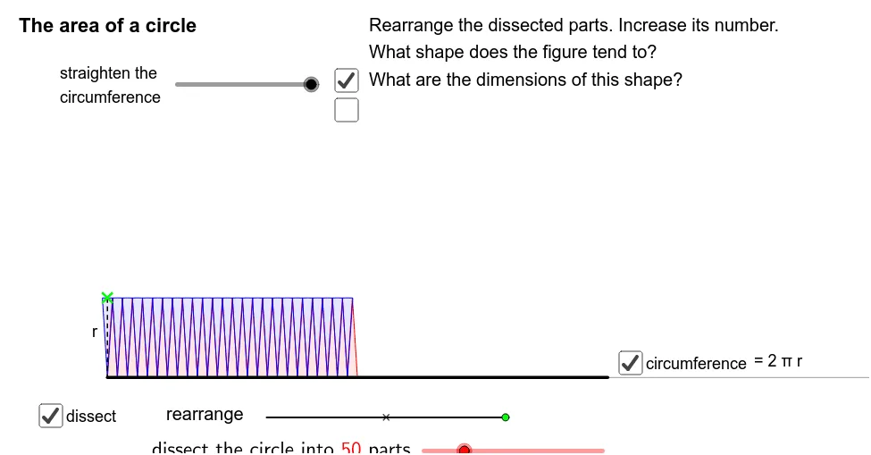
This GeoGebra example demonstrates a dynamic dissection proof of the circle area formula A=πr² and circumference formula C=2πr. It visually shows how a circle can be sliced into sectors and rearranged into an approximate parallelogram or rectangle, whose area and perimeter approach the true values as the number of slices increases. Core concepts include limits, sector and arc length, the geometric meaning of π, and the method of exhaustion. The construction uses commands such as Sequence, Rotate, Sector, Arc, CurveCartesian, and Slider to control the number of divisions n. Objects like Min, Max, Midpoint, Intersect, and dissect are employed to build the dynamic rearrangement. Suitable for middle and high school mathematics, this example helps students intuitively grasp the derivation of circle formulas and introduces foundational ideas of calculus.
GeoGebra Commands & Parameters
Segment(E, (x(E) + 3, y(E))) → aPoint(a) → FMin((x(F) - x(E)) / (a / 2), 1) → kPoint(yAxis) → OSequence(If[k < 1, (x(O) + ((l * sin((i * φ))) * cos((i * φ)) / sin(φ)), y(O) + ((l * sin((i * φ))) * sin((i * φ)) / sin(φ))), (x(O) + (l * i), y(O))], i, 0, (2 * n)) → list2Sequence((x(O) + sin((i * θ)), y(O) + 1 - cos((i * θ))), i, 0, (2 * n)) → list1Max((x(F) - x(E)) / (a / 2) - 1, 0) → k'Rotate((x(O) + 0, y(O) + 1), ((-k) * θ / 2), O) → ARotate(O, ((-k) * θ / 2), O) → O'Rotate(Element[list1, 1], ((-k) * θ / 2), O) → BSector(Rotate[Circle[(x(O) + 0, y(O) + 1), O], ((-k) * θ / 2), O], Rotate[O, ((-k) * θ / 2), O], Rotate[Element[list1, 1], ((-k) * θ / 2), O]) → cRotate((x(O) + 0, y(O) + 1), ((-k) * θ / 2), O) → CRotate(O, ((-k) * θ / 2), O) → O'_1Rotate(Element[list1, 1], ((-k) * θ / 2), O) → DArc(Rotate[Circle[(x(O) + 0, y(O) + 1), O], ((-k) * θ / 2), O], O'_1, D) → dCurveCartesian(t - sin(t), 1 - cos(t), t, 0, 6.28319) → bCircle((0, 1), 1) → hRay((0, 0), (1, 0)) → iPoint(Segment[(0, 1), (6.28319, 1)]) → HSegment(H, (x(H), 0)) → jMidpoint(j) → IMidpoint(a) → JCircle(L, 1 / (1 - m)) → pCircle((0, 0), 1 / (1 - m)) → qIntersect(p, q, 1) → MCircle((0, 1), 1) → c_1Segment((0, 0), (6.283185307179586, 0)) → eSegment(G, (x(G), y(G) - 1)) → rSequence(Sector[Rotate[Translate[Circle[(x(O) + 0, y(O) + 1), Element[list1, i]], Vector[Element[list1, i], Element[list2, i]]], (((-((2 * i) - 1)) * k) * θ / 2), Element[list2, i]], Rotate[Translate[Element[list1, i], Vector[Element[list1, i], Element[list2, i]]], (((-((2 * i) - 1)) * k) * θ / 2), Element[list2, i]], Rotate[Translate[Element[list1, i + 1], Vector[Element[list1, i], Element[list2, i]]], (((-((2 * i) - 1)) * k) * θ / 2), Element[list2, i]]], i, 1, n) → list3Sequence(Sector[Rotate[Rotate[Translate[Circle[(x(O) + 0, y(O) + 1), Element[list1, i]], Vector[Element[list1, i], Element[list2, i]]], (((-((2 * i) - 1)) * k) * θ / 2), Element[list2, i]], (180° * k'), (x(O) + (n * l) - sin(θ / 2) / 2, y(O) + cos(θ / 2) / 2)], Rotate[Rotate[Translate[Element[list1, i], Vector[Element[list1, i], Element[list2, i]]], (((-((2 * i) - 1)) * k) * θ / 2), Element[list2, i]], (180° * k'), (x(O) + (n * l) - sin(θ / 2) / 2, y(O) + cos(θ / 2) / 2)], Rotate[Rotate[Translate[Element[list1, i + 1], Vector[Element[list1, i], Element[list2, i]]], (((-((2 * i) - 1)) * k) * θ / 2), Element[list2, i]], (180° * k'), (x(O) + (n * l) - sin(θ / 2) / 2, y(O) + cos(θ / 2) / 2)]], i, n + 1, (2 * n)) → list4CircleArc((0, 1 / (1 - m)), O, L) → s
AI Drawing Prompt Reference
Create a dynamic visual proof of circle area and circumference. On the left, a unit circle is divided into many sectors, with a slider controlling the number of divisions. On the right, these sectors are rearranged into an approximate rectangle, whose base length approaches half the circumference and height approaches the radius. Also show a cycloid curve and a horizontal segment for comparing arc length with straight length. As the number of sectors increases, the arrangement converges to a rectangle, illustrating the limit process for the area formula.
The prompt above was compiled from the original drawing commands and is for reference only.