Geometric Illustration of Conic Eccentricity via Cone–Plane Intersections

Loading the math board and drawing, please wait…

2021-03-19 20:39

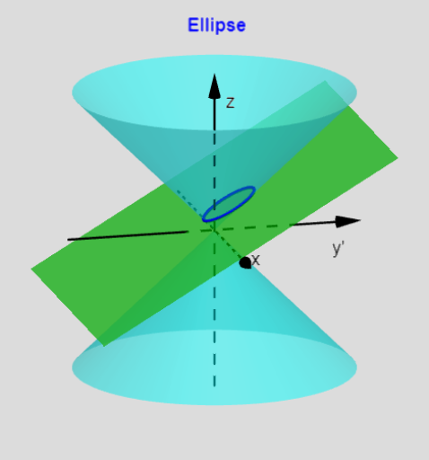
This GeoGebra example visualizes how the eccentricity e determines the “shape” of conic sections by constructing conics as the intersection of a cone with a plane. It demonstrates the geometry behind the ellipse/parabola/hyperbola continuum using spatial angle settings (e.g., θ_{plane}, θ_{cone} and related parameters) and distance/radius relationships (such as r and r_{cone}) to drive the construction. Key concepts include eccentricity (its geometric meaning), conic-section generation through slicing a cone, and angle-based tools (angle bisectors and perpendicular constructions) that control the resulting curve. Construction highlights: Lines are created with Line, conditional configurations are handled with If, AngularBisector builds key bisectors, and OrthogonalLine together with multiple perpendicular helper objects (e.g., L_perp-type objects) enforces right-angle constraints. Intersections are computed with Intersect and IntersectPath to obtain the contact/trace sets, while Cone and Sphere model the 3D geometry. CurveCartesian is used to render curves derived from parameter relationships, and Circle/Segment provide additional geometric constraints and reference elements. Suitable for high school through early university learners studying analytic/solid geometry, and for lessons that seek an intuitive, parameter-driven understanding of eccentricity and conic construction.

GeoGebra Commands & Parameters

Line((0, 0, 0), (0, r_{cone}, 5)) → L_{cone-r}
If(Z_{int} ≠ 0 ∧ abs(sin(θ_{plane-r})) < 0.9999, true, false) → S_{tandard}
Line(P_{z}, (0, 1, z(P_{z}) + tan(θ_{plane-r}))) → L_{plane}
AngularBisector(L_{plane}, L_{cone-r}) → L_{bis-1}, L_{bis-2}
If(e_{s} ≟ 1, (0, 0, Z_{int} / 2), Intersect[L_{bis-1}, zAxis]) → P_{circle-1}
OrthogonalLine(P_{circle-1}, L_{plane}, y = 0) → L_{perp-1}
If(e_{s} ≟ 1, F_{1par}, Intersect[L_{perp-1}, L_{plane}]) → F_{1}
If(e_{s} > 1, asin(1 / e_{s}), 1) → A_{symp1}
If(S_{tandard}, L_{SLR}^(2), 0) → C_{c}
If(S_{tandard}, ((2 * L_{SLR}) * e_{s}), 0) → C_{y}
CornerThreeD(-1, 11) → Corner1
OrthogonalLine(P_{circle-1}, L_{cone-r}, y = 0) → L_{perp-1a}
Intersect(L_{perp-1a}, L_{cone-r}) → P_{horz-1}
Line(P_{horz-1}, yAxis) → L_{horz-1}
Intersect(L_{horz-1}, L_{plane}) → P_{d1}
Line((0, D_{ist}(y(P_{d1}))), xAxis) → L_{d1-g}
Line(P_{g}, yAxis) → L_{Pg}
Intersect(L_{Pg}, L_{d1-g}) → D_1
Segment(P_{g}, F_{1g}) → L_{PF-g}
Segment(P_{g}, D_1) → L_{PD-g}
Intersect(L_{bis-2}, zAxis) → P_{circle-2}
OrthogonalLine(P_{circle-2}, L_{plane}, y = 0) → L_{perp-2}
Intersect(L_{perp-2}, L_{plane}) → F_{2}
If(S_{tandard}, Distance[P_{circle-2}, L_{plane}], sqrt(-1)) → r_{2}
If(S_{tandard}, Distance[P_{circle-1}, L_{plane}], sqrt(-1)) → r_{1}
Line((0, 0, 0), (0, (-r_{cone}), 5)) → L_{cone-l}
Cone((0, 0, 5), (0, 0, 0), r_{cone}) → C_{cone-top}, C_1, C_3
Cone((0, 0, -5), (0, 0, 0), r_{cone}) → C_{cone-bot}, c, C_2
Intersect(L_{plane}, L_{cone-r}) → P_{r}
Intersect(L_{plane}, L_{cone-l}) → P_{l}
Sphere(P_{circle-1}, r_{1}) → s_{1}
Sphere(P_{circle-2}, r_{2}) → s_{2}
OrthogonalLine(P_{circle-2}, L_{cone-r}, y = 0) → L_{perp-2a}
Intersect(L_{perp-2a}, L_{cone-r}) → P_{horz-2}
Line(P_{horz-2}, yAxis) → L_{horz-2}
Intersect(L_{horz-2}, L_{plane}) → P_{d2}
CurveCartesian((r(θ) * cos(θ)), ((r(θ) * sin(θ)) * sgn(Z_{int})), θ, 0, 6.3) → C_{conic-g}
CurveCartesian((r(θ) * cos(θ)), (((r(θ) * sin(θ)) * cos(θ_{plane-r})) * sgn(Z_{int})) + y(F_{1}), (((r(θ) * sin(θ)) * sin(θ_{plane-r})) * sgn(Z_{int})) + z(F_{1}), θ, 0, 6.3) → C_{conic}
IntersectPath(P_{plane1}, s_{1}) → C_{plane1-s1}
IntersectPath(P_{plane2}, s_{2}) → C_{plane2-s2}
Circle(P_{circle-1}, r_{1}, x = 0) → C_{circle-1}
Circle(P_{circle-2}, r_{2}, x = 0) → C_{circle-2}
If(x(Corner1) ≟ -1, 1, If[x(Corner1) ≟ 0, 3, 2]) → View
If(S_{tandard} ≠ 0 ∧ D ≤ 3, If[PointP < 0, "Show", " Hide"]) → textShowHide
If(D ≤ 3, If[PointP < 0, " Point P", " Point P"], "Point P") → textP
CurveCartesian((r(θ) * cos(θ)), (((r(θ) * sin(θ)) * cos(θ_{plane-r})) * sgn(Z_{int})) + y(F_{1}), (((r(θ) * sin(θ)) * sin(θ_{plane-r})) * sgn(Z_{int})) + z(F_{1}), θ, A_{symp1m}, A_{symp1p}) → C_{conic1}
CurveCartesian((r(θ) * cos(θ)), (((r(θ) * sin(θ)) * cos(θ_{plane-r})) * sgn(Z_{int})) + y(F_{1}), (((r(θ) * sin(θ)) * sin(θ_{plane-r})) * sgn(Z_{int})) + z(F_{1}), θ, A_{symp2m}, A_{symp2p}) → C_{conic2}
Line((0, 0), ((-A_{rslope}), 1)) → L_{degm-g}
Line((0, 0, 0), ((-x_{deg}), cot(θ_{plane-r}), 1)) → L_{degm}
Line((0, 0), (A_{rslope}, 1)) → L_{degp-g}
Line((0, 0, 0), (x_{deg}, cot(θ_{plane-r}), 1)) → L_{degp}
If(θ_{plane} ≠ 90, z = Z_{int} + (tan(θ_{plane-r}) * y), y = 0) → P_{plane}
Line(P_{d1}, xAxis) → L_{d1}
Line((0, D_{ist}(y(P_{d2}))), xAxis) → L_{d2-g}
Line(P_{d2}, xAxis) → L_{d2}
If(e_{s} ≤ 1, "+", "-") → signQ
If(Z_{int} ≤ 0, "+", "-") → signL
If(S_{tandard}, If[e_{s} ≟ 0, " Circle ", e_{s} < 1, " Ellipse ", e_{s} ≟ 1, " Parabola ", "Hyperbola"], e_{s} < 1, " Point ", e_{s} ≟ 1, " Line ", "Two Lines") → ConicName

AI Drawing Prompt Reference

Create a 3D geometric illustration showing how eccentricity determines the type of conic via cone–plane intersections. Build two cones (top and bottom) sharing the same apex and add a slicing plane defined by a plane inclination angle, along with key spatial reference axes. Use an angle bisector and perpendicular constructions to locate circle centers by intersecting the bisector direction with the z-axis, then compute two sphere/circle radii based on distances from those centers to the slicing plane. Intersect the slicing plane with the cones to obtain trace/contact sets, and render conic curves using parameter-based Cartesian curve definitions that switch between branches depending on whether eccentricity is below or above 1. Combine the resulting curves and intersection traces to visually communicate the cone-slicing origin of the ellipse/parabola/hyperbola family.

The prompt above was compiled from the original drawing commands and is for reference only.