
Geometric Distribution: PDF and CDF
Loading the math board and drawing, please wait…
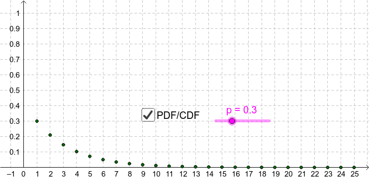
This example demonstrates the probability mass function and cumulative distribution function of a geometric distribution. By adjusting parameter p, users can observe the distribution shapes under different probabilities. The construction uses commands like Sequence and Segment, suitable for high school probability and statistics education.
GeoGebra Commands & Parameters
Sequence(k, k, 1, N) → list1Sequence(p * (1 - p)^(k - 1), k, 1, N) → list2Sequence((Element[list1, k], Element[list2, k]), k, 1, N) → list3Sequence(Sum[Take[list2, 1, k]], k, 1, N) → list4Sequence((k, Element[list4, k]), k, 1, N) → list5Sequence((k + 1, Element[list4, k]), k, 1, N) → list6Sequence(Segment[Element[list5, k], Element[list6, k]], k, 1, N) → list7Segment((-2, 0), (Element[list1, 1], 0)) → aSegment((Element[list1, Length[list1]], 1), (Element[list1, Length[list1]] + 5, 1)) → b
AI Drawing Prompt Reference
Draw a graph showing the probability mass function and cumulative distribution function of a geometric distribution. Use different colors to plot discrete points for the probability mass function and connect them with line segments. For the cumulative distribution function, draw line segments connecting (1,0) to each point of the probability mass function and extend them to the right. Add a vertical line segment from (-2,0) to the first point of the probability mass function and a horizontal line extending 5 units to the right from the last point.
The prompt above was compiled from the original drawing commands and is for reference only.