
Geometric Distribution of Complex Roots of Unity
Loading the math board and drawing, please wait…
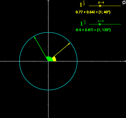
This example demonstrates the geometric distribution of complex roots of unity on the complex plane. It involves core concepts such as complex numbers, polar coordinates, rotation, and vectors. Construction utilizes GeoGebra commands like Circle, Rotate, ToComplex, ToPolar, and Vector to visualize the roots on the unit circle. Suitable for high school or college students studying complex analysis and trigonometry.
GeoGebra Commands & Parameters
Intersect(xAxis, yAxis) → ACircle(A, 1) → cRotate(C, (360 / β)°, A) → NrootAngle(C, A, Nroot) → α_1ToComplex(Vector[Nroot]) → uToPolar(Vector[Nroot]) → vVector(NrootPower) → wToPolar(w) → zAngle(C, A, NrootPower) → β_1ToComplex(w) → aRay(A, w) → hIntersect(c, h) → B,
AI Drawing Prompt Reference
Draw a unit circle centered at the origin on the complex plane. From the origin, draw a ray along the positive real axis intersecting the circle at the point representing 1. Rotate a point on the circle by an angle equal to 360 degrees divided by a positive integer β, obtaining another point on the circle, which is a root of unity. Connect the origin to this point with a vector and display its polar form (magnitude and argument). Then raise this complex number to the power β, yielding a new root of unity; draw its vector and polar representation as well. Finally, draw a ray from the origin through this power point, intersecting the circle, and mark the intersection. The figure illustrates the uniform distribution of roots of unity on the circle and the geometric effect of exponentiation.
The prompt above was compiled from the original drawing commands and is for reference only.