
Geometric Derivation of the Area of a Circle via Sector Rearrangement
Loading the math board and drawing, please wait…
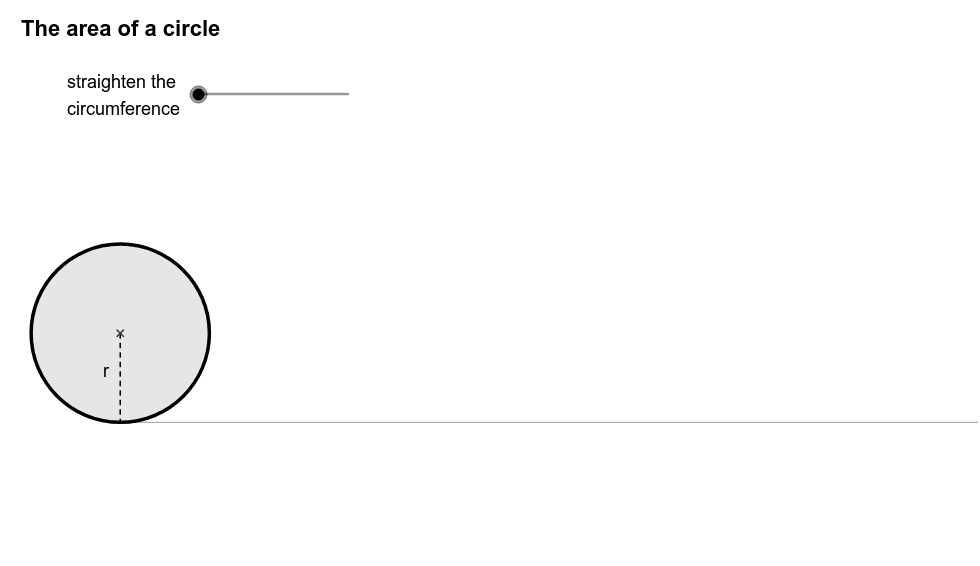
This GeoGebra example dynamically demonstrates the geometric derivation of the area of a circle by cutting it into equal sectors and rearranging them to form a shape resembling a parallelogram, which approaches a rectangle as the number of sectors increases. The core mathematical concepts involved include the area of a circle, the concept of limits (foundational to calculus), geometric transformations (rotation and translation), and the properties of sectors. The construction utilizes key GeoGebra commands such as Sector, Arc, Circle, Rotate, and Sequence to programmatically generate and arrange the sectors, while Segment, Ray, and Midpoint are used to define the boundaries and structural axes. A parameter n controls the number of divisions, illustrating the limit process where the approximated parallelogram's area converges to pi r squared. This tool is ideal for secondary school geometry classes, as well as introductory calculus courses, to provide an intuitive, visual proof of the circle area formula.
GeoGebra Commands & Parameters
Segment(E, (x(E) + 3, y(E))) → aPoint(a) → FMin((x(F) - x(E)) / (a / 2), 1) → kPoint(yAxis) → OSequence(If[k < 1, (x(O) + l * sin(i * φ) * cos(i * φ) / sin(φ), y(O) + l * sin(i * φ) * sin(i * φ) / sin(φ)), (x(O) + l * i, y(O))], i, 0, 2 * n) → list2Sequence((x(O) + sin(i * θ), y(O) + 1 - cos(i * θ)), i, 0, 2 * n) → list1Max((x(F) - x(E)) / (a / 2) - 1, 0) → k'Rotate((x(O) + 0, y(O) + 1), -k * θ / 2, O) → ARotate(O, -k * θ / 2, O) → O'Rotate(Element[list1, 1], -k * θ / 2, O) → BSector(Rotate[Circle[(x(O) + 0, y(O) + 1), O], -k * θ / 2, O], Rotate[O, -k * θ / 2, O], Rotate[Element[list1, 1], -k * θ / 2, O]) → cRotate((x(O) + 0, y(O) + 1), -k * θ / 2, O) → CRotate(O, -k * θ / 2, O) → O'_1Rotate(Element[list1, 1], -k * θ / 2, O) → DArc(Rotate[Circle[(x(O) + 0, y(O) + 1), O], -k * θ / 2, O], O'_1, D) → dCurveCartesian(t - sin(t), 1 - cos(t), t, 0, 6.28319) → bCircle((0, 1), 1) → hRay((0, 0), (1, 0)) → iPoint(Segment[(0, 1), (6.28319, 1)]) → HSegment(H, (x(H), 0)) → jMidpoint(j) → IMidpoint(a) → JCircle(L, 1 / (1 - m)) → pCircle((0, 0), 1 / (1 - m)) → qIntersect(p, q, 1) → MCircle((0, 1), 1) → c_1Segment((0, 0), (6.283185307179586, 0)) → eSegment(G, (x(G), y(G) - 1)) → rSequence(Sector[Rotate[Translate[Circle[(x(O) + 0, y(O) + 1), Element[list1, i]], Vector[Element[list1, i], Element[list2, i]]], -(2 * i - 1) * k * θ / 2, Element[list2, i]], Rotate[Translate[Element[list1, i], Vector[Element[list1, i], Element[list2, i]]], -(2 * i - 1) * k * θ / 2, Element[list2, i]], Rotate[Translate[Element[list1, i + 1], Vector[Element[list1, i], Element[list2, i]]], -(2 * i - 1) * k * θ / 2, Element[list2, i]]], i, 1, n) → list3Sequence(Sector[Rotate[Rotate[Translate[Circle[(x(O) + 0, y(O) + 1), Element[list1, i]], Vector[Element[list1, i], Element[list2, i]]], -(2 * i - 1) * k * θ / 2, Element[list2, i]], 180° * k', (x(O) + n * l - sin(θ / 2) / 2, y(O) + cos(θ / 2) / 2)], Rotate[Rotate[Translate[Element[list1, i], Vector[Element[list1, i], Element[list2, i]]], -(2 * i - 1) * k * θ / 2, Element[list2, i]], 180° * k', (x(O) + n * l - sin(θ / 2) / 2, y(O) + cos(θ / 2) / 2)], Rotate[Rotate[Translate[Element[list1, i + 1], Vector[Element[list1, i], Element[list2, i]]], -(2 * i - 1) * k * θ / 2, Element[list2, i]], 180° * k', (x(O) + n * l - sin(θ / 2) / 2, y(O) + cos(θ / 2) / 2)]], i, n + 1, 2 * n) → list4CircleArc((0, 1 / (1 - m)), O, L) → s
AI Drawing Prompt Reference
Create a dynamic geometry visualization showing how a circle can be divided into equal sectors and rearranged to approximate a parallelogram, leading to the formula for the area of a circle. Draw a circle centered at (0,1) with radius 1. Use a slider to control the number of sectors n. Translate and alternately rotate each sector to form a strip resembling a parallelogram that approaches a rectangle as n increases. Add a horizontal base segment, midpoints, and auxiliary arcs to define the construction boundaries. The overall effect illustrates the limit concept intuitively, suitable for secondary geometry and introductory calculus.
The prompt above was compiled from the original drawing commands and is for reference only.