
Galton Board & Binomial Distribution
Loading the math board and drawing, please wait…
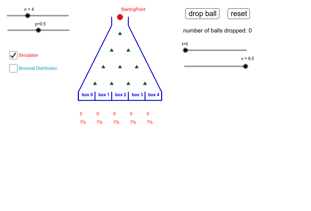
This example uses a Galton board to demonstrate the principles of the binomial distribution. It shows the probability distribution of balls falling into different slots after passing through a series of pins. Key mathematical concepts include the binomial distribution and its probability calculations. Using GeoGebra commands such as Sequence, Join, and Shuffle, the dynamic simulation of the ball's trajectory is achieved. Suitable for high school mathematics education, particularly in probability and combinatorics.
GeoGebra Commands & Parameters
Sequence(Sequence[(i, j), i, j / 2, n - j / 2], j, 1, n) → boardSequence(Polygon[(i - 0.5, 0), (i + 0.5, 0), (i + 0.5, (BinomialDist[n, 1 - p, n - i, false] * h)), (i - 0.5, (BinomialDist[n, 1 - p, n - i, false] * h))], i, 0, n) → BinomialDistJoin({Sequence[-0.5, i, 1, ((10 * n) * (1 - p))], Sequence[0.5, i, 1, ((10 * p) * n)]}) → unshuffleShuffle(unshuffle) → shuffleAppend((n / 2, n + 1), Sequence[(n / 2, n + 1) + (Sum[First[shuffle, i]], (-i)), i, 1, n]) → pathSequence(Segment[(i - 1 / 2, 0), (i - 1 / 2, 1 / 2)], i, 0, n + 1) → containerAppend(Sequence[Segment[Element[path, i - 1], Element[path, i]], i, 1, n + 1], Segment[Element[path, n + 1], Element[path, n + 1] + (0, -1)]) → linePoint(line, t) → PPolyLine(((n - 1) / 2, n + 1), ((n - 1) / 2, n + 0.5), (-0.5, 0.5), (-0.5, 0), (n + 0.5, 0), (n + 0.5, 0.5), ((n - 1) / 2 + 1, n + 0.5), ((n + 1) / 2, n + 1)) → lSequence(Polygon[(i - 1.5, 0), (i - 0.5, 0), (i - 0.5, (Element[rec, i] / Sum[rec] * h)), (i - 1.5, (Element[rec, i] / Sum[rec] * h))], i, 1, n + 1) → box_1Sum(rec) → numberSequence(Text[(Element[BinomialDist, i] / h * 100) + "%", (i - 1.4, -0.4)], i, 1, n + 1) → binopercentSequence(Text[Element[rec, i], (i - 1.4, -0.9)], i, 1, n + 1) → list1Sequence(Text[(Element[rec, i] / number * 100) + "%", (i - 1.4, -1.4)], i, 1, n + 1) → list2Sequence(Text[("box " * i), (i - 0.3, 0.25)], i, 0, n) → boxnumber