
Galton Board & Binomial Distribution by 19sarah88
Loading the math board and drawing, please wait…
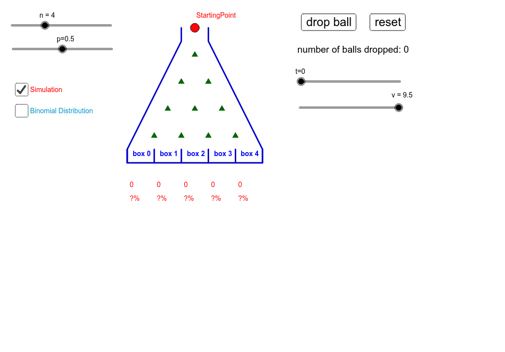
① This interactive GeoGebra example simulates a Galton board (bean machine) to visually demonstrate how falling balls accumulate into a bell-shaped histogram that matches the binomial distribution. ② Core mathematical concepts include binomial distribution, probability mass function, random processes, the central limit theorem intuition, and the connection between discrete and continuous distributions. ③ Construction highlights: using GeoGebra commands such as Sequence, Join, Shuffle, Append, Point, PolyLine, and Sum to generate random paths, draw ball trajectories, and count balls per slot; interactive buttons (button1-4) allow reset, step-by-step, and batch simulations; key objects include n (number of levels), p (probability), BinomialDist (theoretical distribution), and shuffle (random permutation). ④ Suitable for high school to undergraduate probability and statistics courses, ideal for demonstrating how the binomial distribution shape changes with parameters n and p, comparing empirical frequencies with theoretical probabilities, and serving as an entry point for exploring random simulation and statistical inference.
GeoGebra Commands & Parameters
Sequence(Sequence[(i, j), i, j / 2, n - j / 2], j, 1, n) → boardSequence(Polygon[(i - 0.5, 0), (i + 0.5, 0), (i + 0.5, (BinomialDist[n, 1 - p, n - i, false] * h)), (i - 0.5, (BinomialDist[n, 1 - p, n - i, false] * h))], i, 0, n) → BinomialDistJoin({Sequence[-0.5, i, 1, ((10 * n) * (1 - p))], Sequence[0.5, i, 1, ((10 * p) * n)]}) → unshuffleShuffle(unshuffle) → shuffleAppend((n / 2, n + 1), Sequence[(n / 2, n + 1) + (Sum[First[shuffle, i]], (-i)), i, 1, n]) → pathSequence(Segment[(i - 1 / 2, 0), (i - 1 / 2, 1 / 2)], i, 0, n + 1) → containerAppend(Sequence[Segment[Element[path, i - 1], Element[path, i]], i, 1, n + 1], Segment[Element[path, n + 1], Element[path, n + 1] + (0, -1)]) → linePoint(line, t) → PPolyLine(((n - 1) / 2, n + 1), ((n - 1) / 2, n + 0.5), (-0.5, 0.5), (-0.5, 0), (n + 0.5, 0), (n + 0.5, 0.5), ((n - 1) / 2 + 1, n + 0.5), ((n + 1) / 2, n + 1)) → lSequence(Polygon[(i - 1.5, 0), (i - 0.5, 0), (i - 0.5, (Element[rec, i] / Sum[rec] * h)), (i - 1.5, (Element[rec, i] / Sum[rec] * h))], i, 1, n + 1) → box_1Sum(rec) → numberSequence(Text[(Element[BinomialDist, i] / h * 100) + "%", (i - 1.4, -0.4)], i, 1, n + 1) → binopercentSequence(Text[Element[rec, i], (i - 1.4, -0.9)], i, 1, n + 1) → list1Sequence(Text[(Element[rec, i] / number * 100) + "%", (i - 1.4, -1.4)], i, 1, n + 1) → list2Sequence(Text[("box " * i), (i - 0.3, 0.25)], i, 0, n) → boxnumber
AI Drawing Prompt Reference
Draw a Galton board simulation with a triangular array of pegs at the top, where balls drop from the apex and randomly bounce left or right before landing into vertical slots at the bottom. Each slot contains a rectangular bar representing the count of balls, and a theoretical binomial distribution curve is overlaid for comparison. Below the slots, label each slot with its number, actual ball count, actual percentage, and theoretical percentage. Include control buttons for reset, step-by-step, and batch simulation, plus sliders to adjust the number of levels and probability. The overall scene visualizes a statistical experiment.
The prompt above was compiled from the original drawing commands and is for reference only.